Predicting the provisioning potential of forest ecosystem servicesusing airborne laser scanning data and forest resource maps

Jari Vauhkonen

Abstract Background:Remote sensing-based mapping of forest Ecosystem Service(ES)indicators has become increasingly popular.The resulting maps may enable to spatially assess the provisioning potential of ESs and prioritize the land use in subsequent decision analyses.However,the mapping is often based on readily available data,such as land cover maps and other publicly available databases,and ignoring the related uncertainties.Methods:Thisstudy tested the potential to improve the robustnessof the decisionsby meansof local model fitting and uncertainty analysis.The quality of forest land use prioritization wasevaluated under two different decision support models:either using the developed modelsdeterministically or in corporation with the uncertaintiesof the models.Results:Prediction modelsbased on Airborne Laser Scanning(ALS)dataexplained the variation in proxiesof the suitability of forest plotsfor maintaining biodiversity,producing timber,storing carbon,or providing recreational uses(berry picking and visual amenity)with RMSEsof 15%–30%,depending on the ES.The RMSEsof the ALS-based predictionswere 47%–97%of those derived from forest resource mapswith a similar resolution.Due to applying a similar field calibration step on both of the data sources,the difference can be attributed to the better ability of ALSto explain the variation in the ESproxies.Conclusions:Despite the different accuracies,proxy valuespredicted by both the datasourcescould be used for a pixel-based prioritization of land use at a resolution of 250 m2,i.e.,in aconsiderably more detailed scale than required by current operational forest management.The uncertainty analysis indicated that maps of the ESprovisioning potential should be prepared separately based on expected and extreme outcomesof the ESproxy models to fully describe the production possibilities of the landscape under the uncertainties in the models.

Keywords:Forestry decision making,Spatial prioritization,Light detection and ranging(LiDAR),Remote sensing

Background

Forestry decision making requires evaluating potential management alternatives with respect to multiple objectives(Kangas et al.2008).A fundamental decision is related to which goods and services to produce:in addition to conventional timber production,the management objectives may be related to maintaining habitats,providing recreational and aesthetic opportunities,and carbon storage or sequestration(e.g.Pukkala 2016).These goods and services are jointly called“multiple uses”(Kangas 1992)or,following Costanza et al.(1997),Daily et al.(1997)and many others,“ecosystem services”of forest. In the following text, I use ESs to abbreviate“Ecosystem Services”, referring most essentially to indicators of forest-related ESs that can be derived from Remote Sensing (RS) or other digital map data as indirect proxies (Andrew et al. 2014). The mapping of these proxies allows spatial prioritization and other spatially explicit analyses of multiple ESs at various scales (e.g. Schr?ter et al. 2014; R?s?nen et al. 2015; Sani et al. 2016; Roces-Díaz et al. 2017). According to reviews(Martínez-Harms and Balvanera 2012; Englund et al.2017) and a collection of case studies (Barredo et al.2015), however, such analyses can be expected to suffer from the lack of standardized terminology, methodology and data. Increased attention should especially be focused on quantifying and communicating the resulting uncertainties to the decision makers in order to make informed decisions(see also Eigenbrod et al.2010;Schulp et al.2014;Foody 2015).Accounting for these aspects,the present study examines the robustness of forest land-use prioritization based on maps of the provisioning potential of forest ESs(Vauhkonen and Ruotsalainen 2017a),i.e.,the fitness of forest patches to provide goods and services typical to the ESs occurring in the studied area,re-considering the methodological and data workflow proposed in the earlier study.

To result in valid conclusions from RS-based decision analyses,the estimates should be accurate already at the level of individual pixels.The use of active RS such as Light Detection and Ranging(LiDAR)is expected to produce more accurate information compared to passive,optical RS(Lefsky et al.2001;Coops et al.2004;Maltamo et al.2006),especially,when using small pixels(e.g.,200 m2as in N?sset 2002).Forest structure and habitat related inventories in particular benefit from the ability of LiDAR to provide three-dimensional information,when operated as Airborne Laser Scanning(ALS;Maltamo et al.2014).Kankare et al.(2015)evaluated the estimation accuracy of biomass attributes based on two different RSsetups in an area closely resembling to that presently studied.According to their results,pixel-level predictions based on coarse to medium resolution satellite imagery had a Root Mean Squared Error(RMSE)of 47.7%of the total biomass,which could be reduced to 25.7%using ALSand local field reference data.The ALS data used were acquired by the land survey,and the availability of such data is increasing due to large-area acquisitions for terrain elevation modelling.Such data have also been used to map attributes related to habitat(Melin et al.2013,2016;Vauhkonen and Imponen 2016),structural(Valbuena et al.2016b;Vauhkonen and Imponen 2016)and aesthetic(Vauhkonen and Ruotsalainen 2017b)propertiesof the forest.

Overall,when various forest ESs are categorized according to a typology such as the Common International Classification of Ecosystem Services(CICES)as in Englund et al.(2017),the potential of ALSfor assessing the suitability of forest areas to provide these ESs can be characterized as:

–Regulation and maintenance services:A very high number of studies indicates that the vegetation height and density profiles produced by ALSare useful for a detailed quantification of variations in above-ground biomass(N?sset and Gobakken 2008;Zolkos et al.2013;Popescu and Hauglin 2014)and,thus,carbon storage(Patenaude et al.2004).Essentially,ALSproduces a three-dimensional description of the forest structure,which can be related to ecological properties such as habitat types(B?ssler et al.2011)or biological diversity in general(Müller and Vierling 2014)and employed to assess suitability of forests to be maintained as habitats for different species(Davies and Asner 2014;Hill et al.2014;Simonson et al.2014).

–Provisioning services:Several studies carried out especially in boreal forest structures indicate ALS data useful for assessing properties related to wood production.Except that the methods listed in the previous paragraphs can be directly used to assess the production potential of bulk biomass,also more detailed predictions of timber assortments(Korhonen et al.2008;Kotamaa et al.2010;Vauhkonen et al.2014;Hou et al.2016)or wood fiber-related attributes(Hilker et al.2013;Luther et al.2014)are possible.Although the yield studies are mostly related to wood-based biomass,there also are examples of improved assessments of the yield of shrub fruits(Barber et al.2016)or edible fungi(Peura et al.2016)based on ALS.

–Cultural services:The applicability of ALShighly depends on the cultural service of interest.For example,several archaeological studies indicate the potential to improve the mapping of historical remains in the forest using an ALS-based digital terrain model.Similar techniques to visualize the terrain(Domingo-Santos et al.2011)or trees(L?m?s et al.2015)could potentially be used to assess the aesthetic properties of the forest.To date,the study of Vauhkonen and Ruotsalainen(2017b),which assessed the preferences on the visual amenity of a forest area based on cuttings simulated to triangulated vegetation point clouds,appears to be the only ALS-based attempt towards this direction.

The use of ALScan thus be motivated by the potential to obtain a better correspondence with forest biophysical attributes and these data may be available for some areas in a similar extent as land cover maps and other publicly available data.Despite the high potential,however,also ALS-based information may yield a high degree of uncertainties,if applied in expert models formulated according to conventionally measured field attributes.For example,the suitability index proposed by Pukkala et al.(2012)to map potential habitats of Siberian jay(Perisoreus infaustus L.)would require estimating the availability of Vaccinium myrtillus(L.)berries and epiphytic lichens for food and nests.Although sub-models to estimate these attributes are presented(Pukkala et al.2012),also those include stand age and site fertility,which are difficult to estimate by ALS.Although some researchers have predicted even understorey-related attributes,the results of Korpela et al.(2012)indicate that direct measures are difficult to obtain due to transmission losses occurring in the upper canopy(see also Maltamo et al.2005)and such estimations would be even more unreliable based on passive optical RS methods.Even the recognition of dominant tree species may be challenging in ALS-based inventories:despite promising results based solely on ALS(?rka et al.2013;Vauhkonen et al.2014),the results of R?ty et al.(2016)suggest difficulties in detecting species,which dominate a minor proportion of an area otherwise homogeneous in terms of the species.

On the other hand,ALS may allow producing other attributes with more relevance from the forest management point of view.For example,forests with multilayered vertical structure can be distinguished based on the data(Zimble et al.2003;Maltamo et al.2005),which can be further employed in detecting the prevailing silvicultural system(Bottalico et al.2014),management intensity (Sverdrup-Thygeson et al. 2016;Valbuena et al.2016a),or development stage(Valbuena et al.2016b).Even more detailed indices may be developed based on ecological rationale(Listopad et al.2015)or a thorough understanding of the properties affecting the ALS response(Valbuena et al.2013,2014).Earlier studies have suggested that the information in the ALSdata may be condensed to a few metrics(Kane et al.2010;Leiterer et al.2015;Valbuena et al.2017),the partitioning of which will provide a stratification corresponding closely to the structural complexity observed in the field(Pascual et al.2008;Thompson et al.2016;Vauhkonen and Imponen 2016).

Even though properties related to individual ESs have been actively studied,no studies that show how to support management decisions related to the provisioning of multiple forest ESs based on three-dimensional forest structure description obtained by ALS can currently be found from the literature.Barbosa and Asner(2017)and Rechsteiner et al.(2017)derived information from ALS data to prioritize landscapes for ecological restoration and species conservation planning,respectively.Packalén et al.(2011)used ALSdata and spatial optimization to derive so called dynamic treatment units to guide the management of pulpwood production in a plantation forest.Although a similar approach could be extended to the decision making of other or multiple ESs(Pukkala et al.2014),all ALS-based applications are,to date,focused on single ESs.

The purpose of this study is to test ALSdata for management prioritization of multiple ESs in a boreal forest landscape.Proxies for pixel-wise provisioning potential of biodiversity,carbon,timber,berries,and recreational amenities were formulated using ALS-based features and compared to information obtained from forest resource maps with a resolution of 16×16 m2.The quality of land use prioritization based on the obtained information was evaluated under two different decision support models:either using the developed models deterministically or in corporation with the uncertainties of the models.

Methods

A methodological overview

Specifically,the ALS data are tested for predicting the provisioning potential of ESs (Vauhkonen and Ruotsalainen 2017a)in a spatial prioritization framework,where land use decisions are based on ranking the set of decision alternatives in the considered location(s)and choosing the best according to the decision makers’preferences(cf.,Malczewski and Rinner 2015).When applied to prioritize forests for single(e.g.Lehtom?ki et al.2015)or multiple uses (e.g.Vauhkonen and Ruotsalainen 2017a)based on ESproxy maps,a simplified workflow for such analyses includes three methodological steps:

1)Data acquisition,feature extraction and/or expert modelling to derive proxy values for the analyzed ESs.

2)Scaling and normalization of the proxy values derived from different sources to the same scale.The resulting values can be called ‘priority’,‘benefit’,or ‘utility’value and used in different ways depending on the literature source(see also Pukkala 2008;Pukkala et al.2014;Malczewski and Rinner 2015).

3)Decision analyses using the normalized data at selected spatial scale(s).

Because the normalized proxy maps resulting from the previous steps ‘measure’the ESs in a same scale and account for the value range of each ESin the entire landscape,they can be used(a)to mutually rank ESs within a spatial unit to subsequently prioritize management to provide most suitable ESs in each unit;and(b)to identify the most important locations of specific ESs in the landscape to be considered as management hot-spots or cold-spots.Because the spatial prioritization is carried out at a sub-stand-level using pixels or other corresponding map units,it is expected to allow a more efficient use of the production possibilities of the forest(Heinonen et al.2007)and,overall,operationalize the concept of ESs for landscape planning,which is further motivated by de Groot et al.(2010).

The present study examines whether changes to each of the three steps listed above could improve pixel-wise analyses of the provisioning potential of forest ESs(cf.the discussion section of Vauhkonen and Ruotsalainen 2017a):

1) What data to use for the expert models of the provisioning potential: A consolidated approach to obtain grid-based, wall-to-wall predictions for the tessellated landscapes would be to use forest resource maps based on generalizing field sample plot measurements to larger areas using coarse to medium resolution RS images and other numeric map data (Tomppo et al. 2008a, 2008b,2014). This approach, referred to as Multi-Source National Forest Inventory (MS-NFI), was used by Vauhkonen and Ruotsalainen (2017a). Even if ALS allows more prediction possibilities, as reviewed above, it is practically reasoned to benchmark the accuracies against the pixel data provided by the MS-NFI approach, because different forest resource maps are readily available in many countries (Tomppo et al.2008b; Roces-Díaz et al. 2017; Vauhkonen and Ruotsalainen, 2017a).

2) How to scale the ESs originally measured in different units for the joint analyses: Vauhkonen and Ruotsalainen (2017a) used a simple normalization to convert the ES values between 0 and 1:

where vijis the normalized value and nijis the position of the j:th plot in ascending order of the expert model values for the i:th ecosystem service among altogether N plots.Notably,this normalization produced values in an interval scale,whereas the ratios between the expert model values could also be assumed useful for the priority ranking.An alternative,ratio-scale normalization could be computed as:

where vijis the value(or priority or benefit or utility,depending on literature source;see above)produced by the i:th ESin plot j.

3)How to use the obtained information in decision analyses:Vauhkonen and Ruotsalainen(2017a)deterministically prioritized each pixel to the ES with the highest predicted proxy value,but highlighted the need to consider uncertainties around the predictions.If a quantification of the uncertainties is obtained(e.g.,by approximating residual errors of calibration models fitted to the data),the decision analyses can consider distributions of uncertainty in addition to the expected values and produce separate recommendations for different decision makers according to their attitudes towards risk(Pukkala and Kangas 1996).Therefore,in addition to deterministic use of the predicted values,this study considered both the expected and extreme outcomes of the predictions when selecting the most suitable ESfor a pixel.The principal idea of this analysis is illustrated in Fig.1.

On this background,the present study tested the data source(ALS or MS-NFI),priority value function form(Eqs.1 or 2),uncertainty management approach,and joint implications of these choices to the predictions of the provisioning potential of forest ESs and subsequent management prioritization decisions.Forest ESs considered were selected based on two criteria:likelihood to occur in the studied landscape and existence of expert models to derive proxies for their provisioning potential based on the field measurements(Table 1).The field and MS-NFI data contained estimates of forest attribute that could be directly inserted to the expert models.Using ALS data,regression analyses were employed to estimate predictive relationships between ALS-features and ESproxy values to fully utilize the different properties of these data(cf.,Section“ALS-based models for the priority valuesof the ESs”below).In the absence of independent,wall-to-wall data for validation,both the predictions and validations were carried out at the level of individual forest plots.The evaluation is therefore limited to the local fitness of the ESs for a specific forest patch in a single point in time and without considering their spatial or temporal continuum.No decision maker was assumed in this study and the values obtained from both the Eqs.1 and 2 were therefore treated with equal weights,even if those could additionally be weighted according to the decision makers’preference structure.

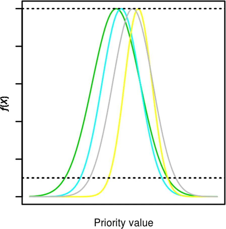
Fig.1 A generic example of selecting the best decision alternative based on different outcomesof modelpredictions(colored curves).The yellow curve yieldsthe highest priority value based on the expected(upper horizontal line)or worst outcome of the model.However,if the decision maker weightsbest possible outcomes,the alternative depicted by the grey curve should be selected asit producesthe highest priority in the right tail accumulation point(the interception of the curve and the lower horizontalline)

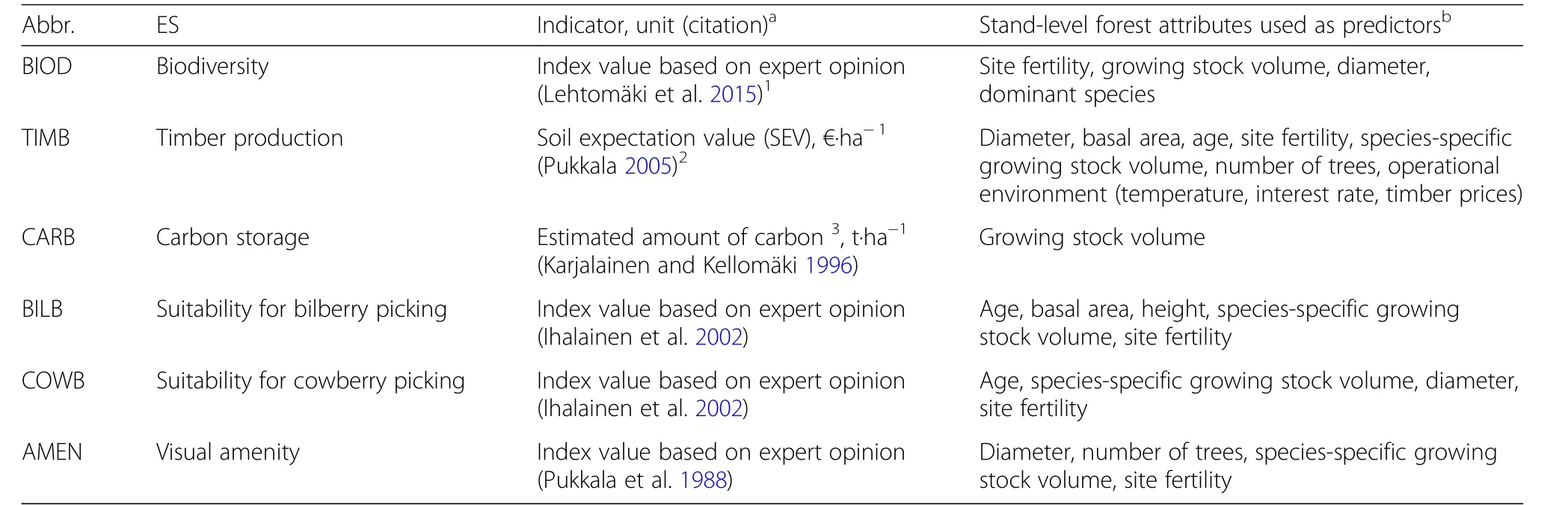
Table 1 The ESs considered in this study and expert models for deriving their reference proxy values

Study area and experimental data

The study area is located in Evo,Finland(61.19°N,25.11°E),which belongs to the southern boreal forest zone.The data extended over an area of approximately 3 km×6 km.The forest stands in the area vary from intensively managed to natural forests in terms of their silvicultural status.Approximately 84%of the growing stock in the studied plots is dominated by coniferous tree species Scots pine(Pinus sylvestris L.)and Norway spruce(Picea abies[L.]H.Karst.).Deciduous tree species such as birches(Betula spp.L.),aspen(Populus tremula L.),alders(Alnus spp.P.Mill.),willows(Salix spp.L.),and rowan(Sorbus aucuparia L.)occur in mixed stands and below the dominant canopy.

Data sets used were compiled from three earlier studies in the same area(Vauhkonen and Imponen 2016;Niemi and Vauhkonen 2016;Vauhkonen and Ruotsalainen 2017a).Vauhkonen and Imponen(2016)downloaded and processed ALSdata acquired by the National Land Survey of Finland to stratify the area according to forest structural properties.The ALSdata were acquired from a flying altitude of 2200 m using Leica ALS 50 scanner on 7 May,2012,to yield a nominal pulse density of 0.8 m?2.Circular sample plots(9 m radius)were placed by clustering the ALSdata with respect to forest structural features,which was found to be an efficient strategy to distribute the sample across the spatial,size,and age distributions of the tree stock(Vauhkonen and Imponen 2016).The field measurements were carried out in June–August, 2014. The species and diameter-at-breast height(DBH)were measured for each tree with a DBH≥5 cm.For each tree species of the plot,a tree with a DBH corresponding to the median tree was measured for height and used to calibrate height curves for predicting the missing tree heights.Plot-level forest attributes were computed from the tree-level measurements using standard equations and methods,which are described in detail in an open-access article by Niemiand Vauhkonen(2016).

Publicly available MS-NFI data(Natural Resources Institute Finland 2017)were included to provide a benchmark for the ALSdata.The MS-NFI maps are the same used Vauhkonen and Ruotsalainen(2017a)and details on their pre-processing are given in that paper.These raster maps depicted site fertility,growing stock volume and biomass components by tree species,total basal area and mean diameter and height corresponding to those of the(basal area weighted)median tree,and they were produced using a k-nearest neighbor(k-NN)estimation method based on optimized neighbor and feature selection(Tomppo and Halme 2004;Tomppo et al.2008a,2014).The method used various satellite images from 2012 to 2014 and National Forest Inventory(NFI)field plot measurements from 2009 to 2013,which were updated to correspond the situation in mid-2013 using growth models.

Altogether 102 field plots were covered by both ALS and MS-NFI data and were included in the analyses.The models of Table 1 were applied to produce plot-specific reference values for the provisioning potential of the ESs based on field data.According to an exploratory analysis,the expert models of Table 1,fit with many different data sets,had considerably different value ranges over the landscape.As a result,a direct normalization of the expert function values specifically with Eq.2 resulted to emphasizing one ESin the priority rankings only because of the different shape and scale of initial value distributions,as elaborated upon in Appendix 1.For this reason,the expert function values of all ESs were transformed to follow the normal distribution as closely as possible using the Box-Cox-transformation(Appendix 1)prior to applying Eqs.1 and 2.The forest attribute estimates based on the MS-NFI maps were transformed using the same parameter values as with field data.This transformation did not affect the order of the observations,but produced approximately equally shaped frequency distributions of every ES,as detailed in Appendix 1.

ALS-based models for the priority values of the ESs

Prediction models with independent variables extracted from the ALS data were formulated to predict priority function values of the form of Eq.2.Priority function values corresponding to Eq.1 were obtained by ordering the aforementioned predictions,i.e.,no separate models were constructed for the function form of Eq.2.

As reasoned in the Introduction,the aim was not to model the forest attributes used as the predictors of the expert models,but to identify and quantify such properties of the ALS point clouds that directly explained the variation in the ES proxies.As visualized in Fig.2,the point clouds of the plots with maximum proxy values did not considerably differ between the ESs in terms of the total distributions.However,when height values or proportions were computed separately according to echo categories,ES-specific differences could be pointed out(Fig.2).The features were therefore extracted in echo categories,which were “only echoes”(suffix_only),“first of many echoes”(_first), “l(fā)ast of many echoes”(_last),“first echoes”(_FP),and “l(fā)ast echoes”(_LP),where the last two categories included “first of many”and “l(fā)ast of many”echoes,respectively,with “only echoes”duplicated in both.Fixed height values of 0.5 m,5 m,and below or above an adaptive height value determined as the height of the 60th percentile were used as the thresholds of ground,shrub,and suppressed or dominant canopy,respectively.

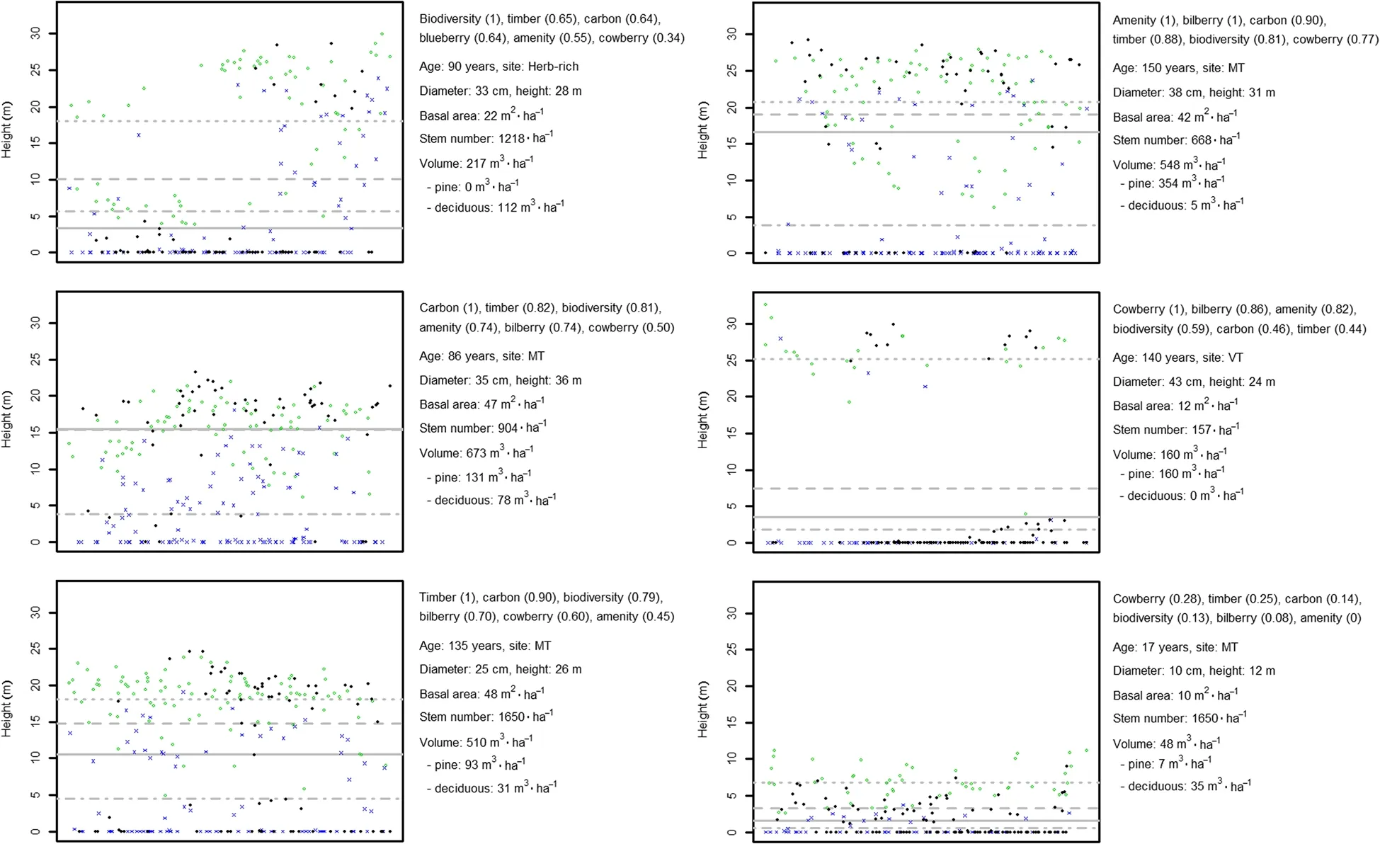
Fig.2 ALSheight profiles and descriptive characteristics of the field plotsconsidered to be most important locationsof the ESsin the data studied(priority value of 1 based on Eq.2).For comparison,the lower right panel shows a plot that had low priority values of the considered ESs.The black,green,and blue symbols indicate only,first-of-many,and last-of-many ALSechoes,respectively.Grey horizontal linesindicate the mean heightsof these echo categoriesand allechoesand are drawn to illustrate the differencesin termsof these metricsbetween the ESs

The following categories of the features were considered:

–Canopy height and density,which are the basic predictors used in ALSanalyses(N?sset 2002)and were assumed to discriminate between size-specific attributes of the ESs:the maximum(hmax),the mean(hmean),and the standard deviation(hstd)of the height values above the ground threshold;the 5th,10th,20th,...,90th,and 95th percentiles(hzz,where zz denoted the percentile value);and the corresponding proportional densities(dzz)were computed according to Korhonen et al.(2008,pp.502–503).

–Proportion of echoes above a given threshold to all echoes,corresponding to a vegetation cover estimate(Korhonen et al.2011).Thisproportion wascomputed in two ways:using echoes of different categories above theground(ccX_ground,where X istheecho category)or first echoesabovetheshrub layer threshold(ccshrub),which correspondsto an attempt to quantify theshrub layer thickness(cf.,Vauhkonen and Imponen 2016).

–Absolute differences between mean heights of different echo categories.These features were computed without height thresholds and assumed to discriminate between properties related to coniferous-or deciduous-dominated forest in the ALSdata acquired during the leaf-off period(Liang et al.2007).These features are denoted by diffx–y,where suffix x–y refers to the height difference of echo categories FP–LP,only–LP,first–only,or first–last.

–Proportions of the different echo categories,which were assumed to be affected by the species and size specific ESproperties in the canopy similar to the ALS-intensity features(?rka et al.2012;Vauhkonen et al.2014).These features are denoted by propX/Y_z,where X/Y indicated the ratio of two echo categories X and Y,and z was the height threshold employed for computations.

–Predictors related to the shrub and understorey layers(Vauhkonen and Imponen 2016):the ratio of the echoes reflected above ground but below the dominant canopy threshold(runderstory);the standard deviation of the height values of echoes reflected above ground but below the dominant canopy threshold(stdunderstory);and the ratio of the echoes reflected from the shrub layer to all echoes(rshrub).

Features xi,i=1,2,…,143,listed above formed the initial set S1of candidate predictors.To account for useful interactions between the features,the final set S was obtained aswhich resulted to altogether 10,296 candidate features per plot.Separate models for each ES were constructed by inserting features iteratively into a model template:

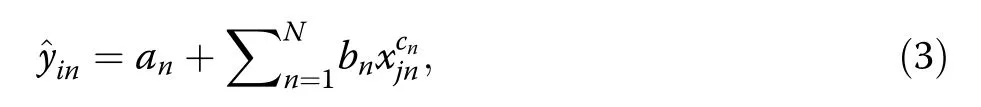
where n is the number of observations,andand yiare the predicted and reference values,respectively.The feature that minimized the RMSE was retained in the model template and the iterations were continued until the model included a maximum of four features.However,more criteria were employed to select the model to be used for the prioritization analyses among the models with one to four features:

1)The final predictor inserted had to improve the RMSEby at least 1%.

2)The residual errors had to satisfy the null hypothesis that the considered sample came from a normally distributed population,which was examined graphically using scatter,residual and QQ-plots,and numerically using the test statistic proposed by Shapiro and Wilk(1965).

3)The model had to pass a“sensitivity of convergence”test,in which the model was fit separately for each plot using Leave-One-Out-Cross-Validation(LOOCV),i.e.,not allowing the plot in question to be available in the training data for model fitting.Implications of including this test are further described in the Results section.

Predicting the priority values of the ESs based on the MS-NFImaps

Benchmark predictions for those based on ALSwere obtained by inserting the forest attribute estimates from the MS-NFI maps to Eq.2.Priority function values corresponding to Eq.1 were obtained by ordering the aforementioned predictions (cf.,previous section).The MS-NFI maps included estimates of all other independent variables except the number of trees per hectare,which was estimated by dividing the total basal area by the basal area corresponding to the mean diameter,i.e.,assuming that the resulting number of average-sized trees existed in a pixel.To compute plot-wise estimates,the pixels of the forest resource maps intersecting with the plot polygons were identified using a spatial query.The estimates of a plot were obtained from the intersecting pixels as weighted averages with the joint areas of the plots and pixels as the weights.Finally,to see if amending the models based on ALS with the MS-NFI layers improved the models,a similar feature selection as with ALS data was run including all MS-NFI-based ES and forest attribute proxies as additional feature candidates.

Field calibration and evaluation of the predictions

Following the method described in the previous section,potential estimation errors in the MS-NFI maps propagate to the predicted priority values,whereas similar error propagation is avoided in the ALS-based analyses due to local model fitting.An additional calibration step was therefore included to eliminate the contribution of the local field sample to the predictions.Calibration models,where yiwas the reference priority value of the i:th ES andits RS-based estimate,of all ESs were fit simultaneously as systems of linear equations.Due to the high inter-correlations(see Additional file 1,Table S1),the models were fit in two steps:first,using Ordinary Least Squares(OLS)to produce model residuals,and second,using Seemingly Unrelated Regression(SUR)to account for the residual error covariance matrices in the final models.The computations were carried out in the LOOCV mode using the systemfit package of R(Henningsen and Hamann 2007).The accuracies of the ALS-and MS-NFI-based predictions were compared using the RMSE and coefficient of determination(R2)computed between the reference values and predictions obtained from the LOOCV models.

Decision analyses

The effects of the aforementioned prediction accuracies to the management decisions were evaluated by comparing the priority ranking of the ESs in each individual plot.The ES with the highest priority value,based on Eqs.1 or 2 applied to the field reference data,was assumed to be the most suitable ES for the specific plot.The RS-based decision was considered correct,if the most suitable ES based on the field data and the RS prediction equaled.The degree of incorrect decisions was quantified using two approaches.First,the correctness of every decision was given a numerical score(Gopal and Woodcock 1994):situations where RS and field data resulted in the same decision was given a score of 6;those where the RS-based service was the second best according to the field data a score of 5;and so on,until the situation where the RS-based service was the worst according to field data,which was given a score of 1.The distributions of these “decision scores” were compared between the different data sources.Second,the dispersion in field and RS-data between the services selected as the most suitable for the specific plot was examined using confusion matrices.The priority ranking of the less important ESs was not evaluated.

In addition to ‘deterministic’decision making described above,the sensitivity of the decisions was examined by incorporating the uncertainties of the models to the analyses(Fig.1).Instead of using the expected values of the priority functions,the ranking was carried out assuming the predictions as realized values of a random variable X～N(E,s2),where E was the expected value and s2was the mean squared error of the model residuals.A similar priority ranking as with the expected values was carried out with predictions that were among the worst and best outcomes of the model,obtained as the values of the 5th and 95th percentiles of the distribution of X of each ES.

Results

ALS-based models for the priority values of the ESs

The ALS features considered as the predictors of the regression models are listed in Table 2.All feature and echo type categories and a wide range of different height values was employed when building the models,for which reason only a few specific observations on the structure of models can be made.All features selected were products of form feature1×feature2,where feature1was often an absolute height value(a mean height,percentile,or height difference)and feature2a proportion (either a canopy cover proxy or proportional density).This combination was especially frequent among the first features selected to the models.In the models of TIMB,all selected predictors were such combinations employing various height values and echo categories.The models of BIOD and CARB used proportion×proportion types of interactions and the ratio of first-of-many to only and first returns(propfirst/FP_ground).The predictors of BIOD(e.g.,propfirst/FP_ground;diffonly–LP;hstdLP)were most diverse in terms of describing the canopy structure with features from different categories.The models of BILB,COWB,and AMEN differed from those mentioned above in employing low percentile values,last pulse proportions and features such aspropfirst/FP_ground, andOverall,the canopy cover proxies were the most frequent feature type,whereas the computing heights and echo categories of all features varied.Although a wide range of different height values was used,a predictor with a percentile value above 70 was selected only once.

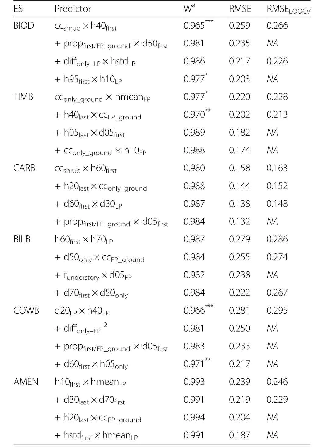
Table 2 The features and performance of ALS-based models for predicting ratio-scaled ESproxy values.W–Shapiro-Wilk test statistic

The graphical assessment of model residuals(detailed results not shown)was mainly in line with the test on residual normality(Table 2):the QQ-plots showed heavy-tailed residuals especially for the models with statistically significant values of the Shapiro-Wilk test statistic.However,the deviations of normality were typically related to one or two plots with the highest or lowest values,and not considered problematic for the further analyses.When examined in the same data used for constructing the models,the performance of every model could be slightly improved by increasing the number of predictors to the maximum number allowed.However,when the models were re-fit using LOOCV,model parameters could not be solved for at least one of the plots in the data,resulting to NA values for this performance factor in Table 2.Although this effect could probably have been avoided by allowing a slightly wider range of initial parameters when fitting the models,it was also considered as a sensitivity issue reflecting an over-parameterization of the initial model to certain types of forest structures.

The volume of deciduous trees and the MS-NFI based proxy for BILB would have replaced the last ALS-based features in the models of CARB and BILB,respectively,and in the models of COWB,the corresponding MS-NFI proxy would have been selected as the second feature.However,none of the aforementioned MS-NFI features performed better than the ALS-features of these models in terms of the feature selection criteria.Based on the considerations above,the ALSand MS-NFI data sets were always used separately.Also,a different number of predictors was used in the ALS-based models for the priority ranking:BIOD and COWB were modeled using only one predictor(the one selected first);TIMB,BILB,and AMEN using two predictors(those selected first and second);and CARB using three predictors selected first.

Comparison of ALSand MS-NFIfor predicting the priority values of the ESs

The models based on ALS data always outperformed those based on forest attribute estimates derived from the MS-NFI maps.As shown in Figs.3 and 4,the ALS-based models generally explained more variation in the ES proxies.The regression lines of the MS-NFI data based on the SUR calibration models also differed more severely from the 0–1-lines.Using MS-NFI data,TIMB was predicted most accurately with an RMSE of 30.4%.The RMSEs of other ESs were also close(30.6%–33.2%),except AMEN,which had an RMSE of 40.5%and BIOD,which was predicted worst with an RMSE of 41.6%.Using ALS,the ES predicted worst(COWB)had an RMSE of 29.8%,which is 97%of the RMSE of the corresponding MS-NFI prediction.The RMSEs of all other ESs were in order of 21.7%–27.5%(57%–83%of the RMSEs of MS-NFI predictions),except CARB,which was predicted most accurately with an RMSE of 15.1%(47%of the RMSE of MS-NFI prediction).The degree of determination of CARB also improved most due to using ALS instead of MS-NFI,from R2=0.11 to 0.81.The R2-improvements of the other ESs were close to this magnitude,except for BILB and COWB,which had R2values close to each other based on both the data sources.The residual errors of models based on ALSand MS-NFIwere somewhat correlated for BILB and COWB,but not for the other ESs(Figs.3 and 4,right column).

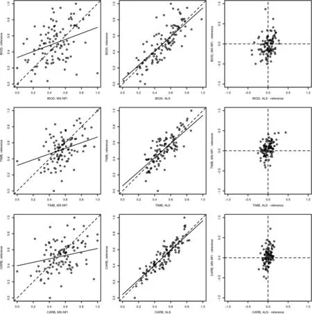
Fig.3 Predicted(x-axis)versus reference priority values of BIOD(upper row),TIMB(middle row)and CARB(bottom row)based on MS-NFI(left column)or ALS(middle column).The broken and solid lines are the 1:1 line and regression line of the SURcalibration models fit with the local field sample,respectively.The right column shows the residuals of the corresponding predictions based on ALS(x-axis)and MS-NFIdata

Decision analyses based on different priority functions,data,and model uncertainties

Compared to the use of interval-scaled priority functions,those based on the ratio scale slightly increased the proportion of decisions that had a perfect agreement in both ALSand field data(Fig.5,left panel).The same observation was made regarding the decisions based on the MS-NFI data,but the differences between the priority function forms were in general minor.When the ratio-scaled priority functions were used in the remaining analyses,the ALS and field data resulted to the same decision in 42%of the plots;the ALS-based ES was at least the second best according to field data in 69%;and among the three best alternatives in 84%of the plots.With MS-NFI data calibrated by the local field sample,the corresponding figures were 46%,61%,and 72%and slightly lower without the calibration,the distribution of the decision scores of all data sources being shown in Fig.5(right panel).Thus,although the calibrated MS-NFI data did better in selecting ESs that matched perfectly with the field data,the proportion of poorest decisions was considerably lower based on the ALS data.The ALS-based models resulted to a better decision in 32%,those based on the MS-NFI data in 27%,and the decision equaled in 41%of the plots.Of the latter group of plots,around 2/3 had either BILB or COWB as the most important ES and the decisions for these plots were generally scored≥4.Except for data sources,the decision score was highly dependent on the priority difference between the best ESs observed from the field plots:in the plots where the decisions equaled between the data sets,the average priority difference between the ESs prioritized as the first and second was 0.12(standard deviation 0.08),whereas the corresponding figures for the other plots were 0.07(0.07).

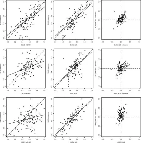
Fig.4 Predicted(x-axis)versus reference priority values of BILB(upper row),COWB(middle row)and AMEN(bottom row)based on MS-NFI(left column)or ALS(middle column).The broken and solid lines are the 1:1 line and regression line of the SURcalibration models fit with the local field sample,respectively.The right column shows the residualsof the corresponding predictionsbased on ALS(x-axis)and MS-NFIdata

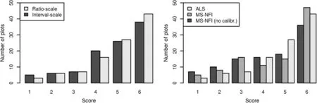
Fig. 5 The distribution of decision scores (left:) between interval- (Eq. 1) and ratio-scaled (Eq. 2) priority functions in ALS data, or (right:) between data source in ratio-scaled priority. Situations where RS and field data resulted in the same decision was given a score of 6; those where the RS-based service was the second best according to the field data a score of 5; and so on, until the situation where the RS-based service was the worst according to field data, which was given a score of 1.

Decision making based on the 5th percentile of the ALS-predicted priority value distributions reduced the proportion of worst decisions(Fig.6,left panel).Otherwise,the decisions based on either the 5th or 95th percentile did not compare favorably with those based on the expected value in either data(Fig.6).The confusion matrices for the most important ESs based on the different data sources and either the expected or extreme outcomes are shown as Appendices 2 and 3,respectively.A comparison of the confusion matrices based on either expected or extreme values indicates that many plots with the most important ES as those predicted with the highest or smallest error rates(e.g.,CARBor COWB,respectively,based on ALSdata)could be prioritized for this ES only by explicitly considering the extreme model outcomes.As a number of plots obtain a different prioritization based on the expected values,it was found interesting to look at the plots for which the prioritization changed depending on the model outcome.Using ALS-based ESproxy models,the prioritization based on the expected,worst,and best outcomes equaled in only 22 plots(in 43 using MS-NFI maps calibrated with the field data).If all decision alternatives based on the three outcomes of the ALS-models were considered,the alternative that matched perfectly with the field data was included in 57%of the plots;an alternative among the two best ones in 85%;and among the three best ones in 93%of the plots.With MS-NFI data,the corresponding figures were 59%,76%,and 88%.Thus,especially the ALS-models were found useful in confining the decision alternatives to those most feasible according to production possibilities,from which the one preferred most preferred according to the stakeholder preferences could be selected based on further MCDA.

Discussion

Earlier RS-based decision analyses of multiple ESs have relied on map scales such as 1:25,000(Roces-Díaz et al.2017)or pixel sizes such as 500×500 m2(Schr?ter et al.2014).Also smaller pixel sizes of 60×60 m2(Lehtom?ki et al.2015)or 48×48 m2(Vauhkonen and Ruotsalainen 2017a)have been used in spatial prioritization analyses.Many of the aforementioned scales are coarse considering the need to formulate management prescriptions at the level of operational units(e.g.,forest compartments),which are typically 1.5–2.0 ha in size in Finland(Koivuniemi and Korhonen 2006).Based on this background,the results of the present study are encouraging:the use of ALS in particular allowed deriving accurate predictions for plots of around 250 m2,i.e.,in a considerably more detailed resolution than current operational compartments.The RMSEs of predicting the studied ES indicators by ALSwere 47%–97%of the RMSEs of corresponding predictions based on benchmark forest resource maps derived using coarse satellite images.Due to applying a similar field calibration step on both of the data sources,the difference can be attributed to the better ability of ALS to explain the variation in the ES proxies.In the sub-sections below,the results are discussed from the points of view of using ALSdata to predict various ESindicator proxies(Table 1)and using these predictions in decision analysescompared to other data.

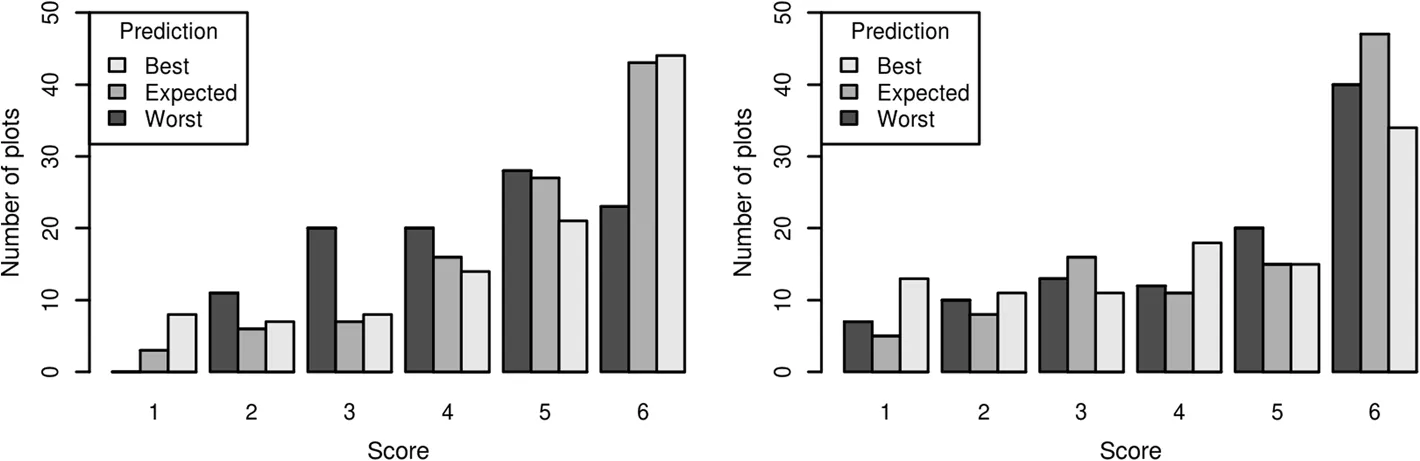
Fig. 6 The distribution of decision scores based on the use of ratio-scaled priority functions and different outcomes of the prediction models in ALS (left) and calibrated MS-NFI data (right). See the caption of Fig. 5 for the interpretation of decision score values.

On the ESproxies and their ALS-based modelling

The expert models(Table 1)express the suitability of forests for the ESs as transformations of forest attributes.Applying the expert models yielded the highest biodiversity conservation values for mature,densely stocked forests.The values were weighted by site fertility such that most fertile sites received a considerable weight compared to poorer sites.An increasing basal area and mean diameter increased the soil expectation value of all the species,but otherwise the model included species-specific interactions between these and operational environment related parameters.The value of carbon storage increased according to an increasing stem volume depending on the species-specific biomass expansion factors.An increasing maturity(measured in terms of mean age and diameter)and decreasing stand density(measured in terms of either basal area or stem number)increased the suitability of a site for berry picking and visual amenity.The latter models also included species-specific terms such that especially the presence of pine trees improved the values.Thus,the response variables of all other ESs except CARB were modelled as functions of multiple forest attributes.

The models based on the ALSdata(Table 2)explained the differences in the provisioning potential of the different ESs with RMSEs of 15%–30%.The selected features and model performances are well in line with the background given in the previous paragraph.The predictions of CARB had the highest accuracies,because those essentially explained the variation in the total stem volume converted to carbon using biomass expansion factors.The ratio of first-of-many to all first echoes(propfirst/FP_ground)was used as a predictor of CARB in addition to height and density metrics,which are typical to total biomass or carbon models.The aforementioned feature has been found useful for separating species(?rka et al.2012;Vauhkonen et al.2014)and should be studied in a broader forest modeling context.Although the field proxy value for TIMB was computed using species-specific predictors,the model based on the ALS data included only features based on height.The models for the other ESs included ALS-based predictors that were clearly related to forest canopy structure:for example,features indicating the existence or abundance of low vegetation were frequently selected to the models of BIOD or recreation-related ESs,respectively.No clear recommendations for the selection of features can be given,except for using multiple heights and echo types when computing the candidate features.The requirement to estimate a high number of model parameters was likely reduced by including products of all candidate features to account for interactions between them,which is a useful property that has not been reported in earlier ALS studies.The features used here are the most common and easily implementable using available software packages such as R.However,it is acknowledged that not all features presented in the literature were included and it could be possible to improve the results with more experimental ones such as those related to volumetric(Vauhkonen and Ruotsalainen 2017b)or textural(Niemi and Vauhkonen 2016)properties.

The proxies listed in Table 1 are measured in different units.In order to use the proxies in decision analyses,those need to be normalized to the same scale,which was done in this paper prior to the modeling.Due to the transformations,the prediction accuracies cannot be easily compared with earlier studies,even in relative scale.Even CARB,which is a species-specific transformation of the total volume,cannot be directly compared to previous studies that predict total biomass or carbon due to the Box-Cox-transformation (Appendix 1) applied to equalize the distribution of the response variables for the decision analyses.If a similar model for CARB had been fit without the Box-Cox-transformation,the RMSE would have risen to around 34%.It is higher than(e.g.)the RMSE of 25.7%obtained by Kankare et al.(2015)for total biomass in the same region,but when comparing the figures the differences in the definition of the response variable and a slightly different plot size must also be considered.For more reasoning on the need for the transformations,please see the next section.On the other hand,the modeling task considered above may have been alleviated by the fact that all response variables resulted from models that had been formulated earlier using common forest mensurational attributes.Actual differences between berry yields of two forests could be much more discrete than those predicted as a function of forest attributes.The performance of the models should thus be tested by re-fitting or validating the models against ES-specific indicators that are not based on models but direct observations made in the field(see also Hegetschweiler et al.2017;Kohler et al.2017).

On the other hand,it may be less feasible or even impossible to predict certain ES properties otherwise than using features quantifying the three-dimensional forest structure.Examples in the Scandinavian boreal forest structures include mammal or bird habitats(e.g.,Melin et al.2013,2016),which could have realistically occurred in the studied area,but could not be included in the present comparison due to the lack of models based on information obtainable from forest resource maps or field plots.The value of ALS data can be seen to lie especially in applications that require identifying sites with high value for e.g.conservation as ALS data coverage is globally increasing and the method has been proven to provide 3D descriptions of vegetation structure that,in turn,have been long known as primary determinants of habitat quality and biodiversity(MacArthur and MacArthur 1961;Dueser and Shugart Jr,1978;Brokaw and Lent,1999).Nevertheless,Vihervaara et al.(2017)identified only four Essential Biodiversity Variables that could benefit from the use of RS data.According to this study,the obtainable improvements are most likely indicator-specific,with magnitude depending on what RS data are available.

Other aspects of RS-based decision analyses:Data,normalization,and uncertainties

This study tested normalization resulting to values in either an interval-(Eq.1)or ratio-scale(Eq.2).Even though the priority value functions based on the different scales did not differ considerably,those based on the ratio-scale performed slightly better in the priority ranking,which is logical as also the ALS-based features provide information at a ratio scale.Although the purpose is not to exhaustively discuss the implications of different value function forms,one important practical aspect discovered in the exploratory analysis could be brought up:An incorrect selection of a value function form would result in biased decisions by weighting the rank-orderings of the alternatives to an undesired direction,which is exemplified by a comparison of the transformed and non-transformed value function forms(Appendix 1).This discussion highlights the importance of considering data normalization procedures in detail already at the modeling stage,if the final applications aim at decision analyses where all modeled proxies should be measurable at the same scale.

The ALS and MS-NFI data sources showed several differences,when predicting the priority value functions.Except having a more deterministic relationship with the forest attributes,one additional improvement of the locally fit ALS models is the ability to predict the 0–1-value ranges directly.When using forest attributes such as those predicted by the MS-NFI,the maximum values used in the normalization should be representative of the entire area.In this study,the minima and maxima predictions based on the MS-NFI were more severely incorrect than with ALS data(Figs.3–4),which partially explains the poorer performance of this data source.Many multivariate predictions from RS data are based on non-parametric nearest neighbor methods,which could have been considered also in the case of ALS data.However,the aforementioned problem would be seriously present also in those types of predictions.

Regardless of the input data or applied scale or mapping technique,it is well recognized that the resulting ES maps will include uncertainties(Eigenbrod et al.2010;Schulp et al.2014;R?s?nen et al.2015).A few earlier spatial prioritization studies(Lehtom?ki et al. 2015; R?s?nen et al.2015;Vauhkonen and Ruotsalainen 2017a)used forest attribute maps in a similar resolution as considered here,but without a calibration based on field data.Such a practice cannot be recommended due to the observed uncertainties in the uncalibrated MS-NFI data in particular.However,it should be acknowledged that all analyses carried out in the aforementioned studies might not be sensitive to incorrect pixel-level prioritization decisions.Also,each of the aforementioned studies used either aggregated pixels to somewhat account for these effects.It is not possible to address the uncertainty reduction due to the use of aggregated resolution based on the field data of this study,which was collected from fixed-size plots.

Finally,it should be noted that in the actual decision making,the stakeholder preferences may affect or even dictate the allocation of the ESs over suitability of forest structure.Even if the decision maker had no preferences on the ESs,aggregating individual pixels,i.e.,deviating from their local optima to compose larger treatment units,could be feasible with respect to the implementations of management prescriptions or achieving ecological or economic objectives that are determined over a larger area(Pukkala et al.2014).Importantly,the decisions based on the same data may differ for a risk-avoiding,risk-neutral or risk-seeking decision maker(Pukkala and Kangas 1996).The risk preferences of the decision maker should clearly be incorporated in the decision making based on the ES maps.Here,a similar technique as in Pukkala and Kangas(1996)was used to account for the uncertainties emerging from different accuracies of the ES proxy models.The results reported in the last paragraph of the Results section can be concluded such that separate forest ES maps should be prepared using the expected,worst,and best outcomes of the model predictions to fully describe the production possibilities of the landscape under the uncertainties in the models.Also those related to the decision makers’preferences could be accounted for as additional stochastic distributions in the analyses(e.g.,Kangas et al.2007)and incorporated in analyses as pixel-level production constraints.Overall,the prioritization approach should be tested further involving real decision makers.

Conclusions

The provisioning potential of ESs(biodiversity,timber,carbon,berries,and visual amenity)was modeled as expert model-based proxies that express the suitability of forests for the ESs as transformations of forest attributes.The models based on the ALS data explained the variation in these proxies with RMSEs of 15%–30%.The RMSEs of the ALS-based models were 47%–97%of the RMSEs of corresponding predictions based on the MS-NFI forest resource maps.Due to applying a similar field calibration step on both of the data sources,the difference can be attributed to the better ability of ALS to explain the variation in the ES proxies.

The RMSE-differences did not fully translate to the accuracies of land use decisions:instead,prioritizing the land use for the ESs with the highest provisioning potential could be done with rather similar accuracies based on both data sources and at a resolution of 250 m2,i.e.,in a considerably more detailed scale than current operational forest management units.ALS-based models for the ES proxies can however be recommended based on their better stability regarding the model errors.The results suggest that separate forest ES maps should be prepared using the expected,worst,and best outcomes of the model predictions to fully describe the production possibilities of forest under the uncertainties in the models.

Additional file

Additional file 1:Empirical cumulative density and probability density function formsand Pearson correlation coefficientsof different transformations of the expert model predictionsfor the ESsconsidered.(DOCX 1758 kb)

Appendix 1

Box-Cox transformation of the reference priority values for the ESs

An exploratory analysis revealed a practical comparability issue related to using the expert function values for the ESs directly in Eq.2,which can be demonstrated by visualizing the empirical cumulative distribution functions and histograms of the data(Additional file 1:Figure S1-Figure S6).The expert functions of Table 1 were fit with many different data sets having different value ranges and resulting to unequal frequencies for the different ESs,when applied in the present data.Using Eq.2,these differences would have translated directly to the priority values,which was found problematic with respect to their ranking.Look especially at the left-hand columns of Additional file 1:Figure S1-Figure S6 and compare Additional file 1:Figure S6 to the others:the direct use of these values would have resulted to a very high number of plots being prioritized as AMEN only because its distribution more frequently included higher values compared to the distributions of the other ESs,which were more often skewed to the left.For this reason,the expert model values of every ES were transformed to produce frequencies that followed the normal distribution as closely as possible prior to converting the value ranges between 0 and 1.The transformation was obtained as(Box and Cox 1964):

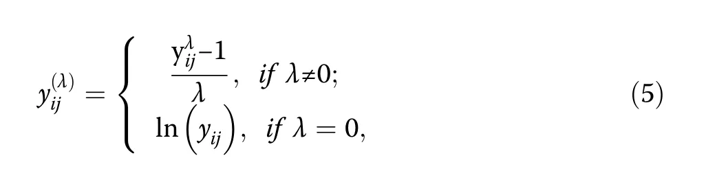
where yijis the original value of the i:th observation of the j:th ES proxy andλis a parameter.The value ofλwas selected from an interval of?3 to 3 as the value that maximized a test statistic on whether the considered sample came from a normally distributed population(Shapiro and Wilk 1965).This transformation did not affect the order of the observations,but produced approximately equally shaped frequency distributions of every ES.As a result,the ESs could be prioritized using two alternative priority value function forms illustrated in the two rightmost columns of Additional file 1:Figure S1-Figure S6:either according to the interval scale(Eq.1)based only on the order of the observations or according to the ratio scale(Eq.2)preserving the ratios between the observations,but thanks to the Box-Cox-transformation,having approximately equal(close to normal)frequency distributions between the ESs.The function forms and frequency distributions of the priority values are shown in Additional file 1:Figure S1-Figure S6 and the correlations between the priority valuesin Additional file 1:Table S1.

During the feature selection process,it was noted that exactly the same features would have been selected to the models,regardless of whether the original or Box-Cox-transformed response variables were used.Therefore,although the Box-Cox-transformation has been rarely used in ALS-based studies,it could potentially aid also other applications by normalizing the response variable to a desired form in the model fitting step.

Appendix 2

Confusion matrices for the most important ESs based on expected outcomes

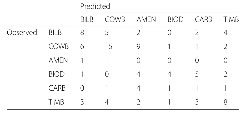
Table 3 Confusion between ESs considered as most important based on the field data(observed)and MS-NFImaps(predicted)using the expected values of the predicted ESproxies

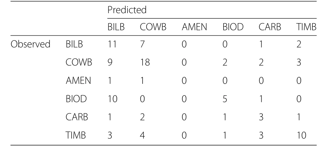
Table 4 Confusion between ESs considered as most important based on the field data(observed)and MS-NFIdata calibrated with the local field sample(predicted)using the expected values of the predicted ESproxies

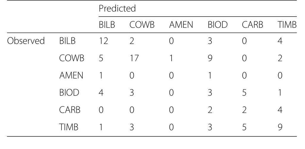
Table 5 Confusion between ESs considered as most important based on the field data(observed)and the expected values of the ALS-based modelsfor ESproxies(predicted)

Appendix 3

Confusion matrices for the most important ESs based on extreme outcomes

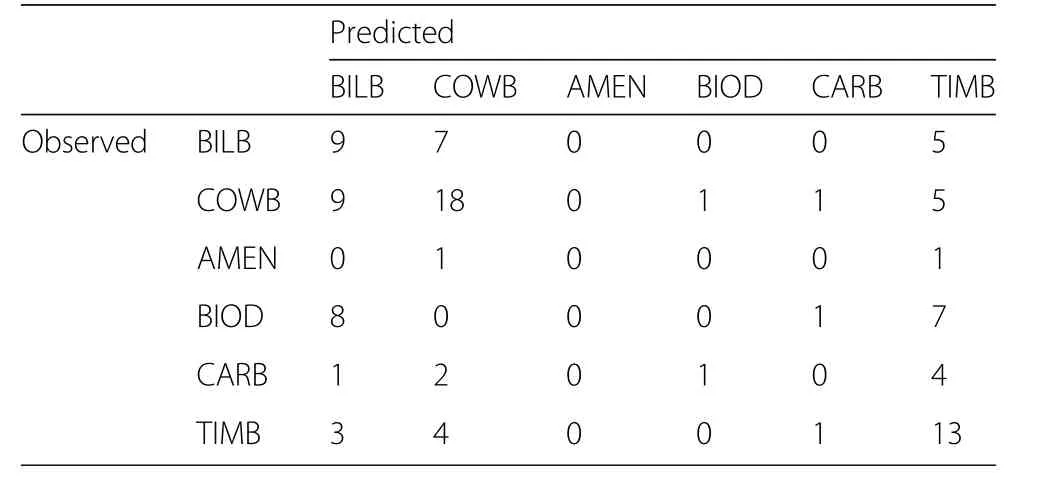
Table 6 Confusion between ESs considered as most important based on the field data(observed)and MS-NFIdata calibrated with the local field sample(predicted)using the worst outcomes of the predicted ESproxies

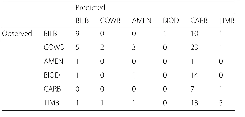
Table 7 Confusion between ESs considered as most important based on the field data(observed)and the worst outcomes of the ALS-based models for ESproxies(predicted)

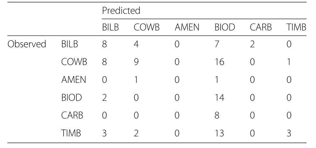
Table 8 Confusion between ESs considered as most important based on the field data(observed)and MS-NFIdata calibrated with the local field sample(predicted)using the best outcomes of the predicted ESproxies

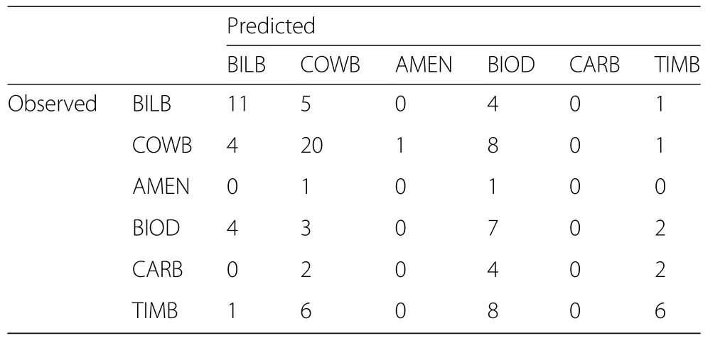
Table 9 Confusion between ESs considered as most important based on the field data(observed)and the best outcomes of the ALS-based models for ESproxies(predicted)

Abbreviations

ALS:Airborne Laser Scanning;AMEN:Visual amenity(one of the ecosystem services considered,see Table 1);BILB:Suitability for bilberry picking(one of the ecosystem services considered,see Table 1);BIOD:Biodiversity(one of the ecosystem services considered,see Table 1);CARB:Carbon storage(one of the ecosystem services considered,see Table 1);COWB:Suitability for cowberry picking(one of the ecosystem servicesconsidered,see Table 1);DBH:Diameter-at-breast-height;ES:Ecosystem service;k-NN:k-Nearest neighbor;LOOCV:Leave one out cross validation;MCDA:Multiple criteria decision analysis;MS-NFI:Multi-Source National Forest Inventory;RMSE:Root mean squared error;RS:Remote sensing;TIMB:Timber production(one of the ecosystem services considered,see Table 1)

Funding

The acquisition of the studied data was originally supported by the Research Funds of University of Helsinki.

Availability of data and materials

All data and materials can be obtained by requesting from the author.

Author’s contributions

JVis the sole author.He carried out all analyses and drafted the manuscript.The author read and approved the final manuscript.

Ethics approval and consent to participate

Not applicable.

Competing interests

The author declares that he has no competing interests.

Received:14 March 2018 Accepted:24 May 2018