Fast Parallel Method for Polynomial Evaluation at Points in Arithmetic Progression

LU Jian-kang,CHEN Hai-biao,JING Rui-xing

(School of Mechanical Engineering,Northwestern Polytechnical University,Xi’an 710072,China)

Fast Parallel Method for Polynomial Evaluation at Points in Arithmetic Progression

LU Jian-kang,CHEN Hai-biao,JING Rui-xing

(School of Mechanical Engineering,Northwestern Polytechnical University,Xi’an 710072,China)

We present a fast method for polynomial evaluation at points in arithmetic progression.By dividing the progression into m new ones and evaluating the polynomial at each point of these new progressions recursively,this method saves most of the multiplications in the price of little increase of additions comparing to Horner’s method,while their accuracy are almost the same.We also introduce vector structure to the recursive process making it suitable for parallel applications.

algorithms;parallel algorithms;polynomial evaluation;Horner’s method

§1.Introduction

Horner’s method is a standard minimum arithmetic method for evaluating and def l ating polynomials.However,in lots of applications,polynomials are evaluated at points in an arithmetic progression[1]and the method presented here is aimed to farther minimum the number of arithmetic operation for those applications.

Normally,a multiplication consumes more time than an addition(subtraction is considered equivalent to addition in this paper)in an algorithm,hence,we can accelerate an algorithm by reducing the number of multiplications.Sometime this reduction is accompanied by an increase of additions.

§2.Horner’s Method

Given a polynomial of degree n

To reduce the number of multiplications,Horner’s method suggests to rewrite(2.1)in a nested form

To solve(2.2),use the following recurrence

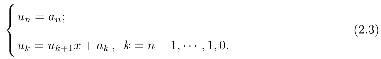
Finally,we have Pn(x)=u0.In general,to evaluate Pn(x)at one point,Horner’s method requires n multiplications and n additions.It is proved that Horner’s method gives a minimum arithmetic evaluation when coefficients of the polynomial are not preconditioned[24].Since Horner’s method is purely sequential,it can not benef i t from parallel hardware.Modif i ed algorithms are introduced for some degree of parallelism in[5-6].However,these parallel algorithms do not have a distinct saving in arithmetic operations.

§3.A Fast Parallel Method

3.1 Problem

Compute Pn(x)at arithmetic progression{xj},where

3.2Fundamental Theorem

By Taylor’s formula with Lagrange remainder

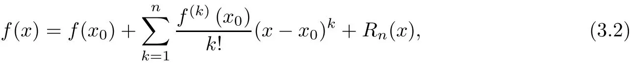
we have f(n+1)(x)≡0 to any polynomials of degree n,hence,expand Pn(xj+1)at xj,we have Rn(x)=0,which means

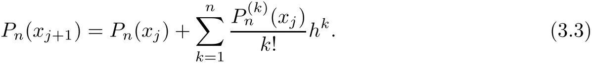
Obviously,the last term of(3.3)is a polynomial of degree n?1 at xj,denote it as Pn1(xj). Moveover,denote Pn(xj)as Pn0(xj),we can rewrite(3.3)as

For easy description,rewrite the formula above as

Similar with the def i nition of P1j,def i ne

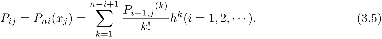
Pijis a polynomial of degree n?i in(3.5),obviously,Pnjis a constant.When i＞n,Pij≡0. According to(3.5)and Taylor’s formula,similar to(3.4),we have

Let j=0 in(3.6),then x=x0=A,we have

Since Pnjare constants,when P00,P10,P20,···,Pn0are computed,we can recursively use(3.6) to compute P0j,i.e.,Pn(xj)(j=1,2,3,···,N).

3.3Procedure

Step 1bir(r=0,1,2,···,n?i)are the coefficients of Pij/hn?i(i=1,2,···,n?1).According to(3.5),compute birby h and coefficients of Pn(x)(terms are arranged by increasing powers of x).The constant term of Pij/hiis

where b0r=ar(r=1,2,···,n).Let

we have

Step 2Pi0/hiare Pij/hi(i=1,2,···,n?1)at x0,which are computed by Horner’s method;secondly,multiply each Pi0/hiby hi,we get P10,P20,···,Pn?1,0and then compute P00by Horner’s method;f i nally compute Pn0as follow

Step 3From(3.4),(3.6)and(3.7),compute Pij(i=1,2,···,n?1,j=1,2,···,N)in a recursive parallel way as follow.

Def i ne vectors

where j=0,1,2···,N?1.

According to the values of P00,P10,···,Pn0in Step 2,compute Pj+1recursively from P0and Q0as

The f i rst entry of Pj+1is P0,j+1,i.e.,Pn(xj+1).

To reduce calculation times,when calculate the latter n?1 values of P0,j+1,redef i ne Pjand Qjas

where k=n?1,n?2,···,1,j=N?k.

Again,we compute all the entries in vector Pjand Qjaccording to(3.13).It saves n(n?1)/2 additions in this new def i nition of Pjand Qj.

3.4The Number of Arithmetic Operations

3.4.1Operation counts in Step 2 and Step 3

In step 3,it costs n(n?1)?n(n?1)/2 additions in total to compute all the P0j(j= N?n+2,···,N)and n additions to compute each P0j(j=0,1,2,···,N?n+1).

In step 2,it costs n(n+1)/2 additions and n(n+1)/2 multiplications to compute all the Pij/hi(i=1,2,···,n?1).

To compute all the hi(i=1,2,···,n?1)recursively and multiply them by Pi0/hi,it costs another 2n?1 multiplications.Thus,computation in Step 2 and Step 3 costs A1additions and M1multiplications,where

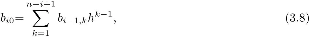
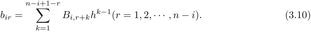
3.4.2Operation Counts in Step 1

Eqs(3.8)and(3.10)are polynomials of h.The degree of(3.8)is n?i,while(3.10)is n?i?r.Apply Horner’s method to compute(3.8)and(3.10)respect to each i and r,it requires A2additions and M2multiplications,where

When i=1,2,···,n?1,r=1,2,···,n?i,coefficients of the polynomial in(3.10)form a series of(n?i)-order symmetric matrixes,denote them as M(n?i).Elements of M(n?i) under their secondary diagonals are zero.Hence,when Crkhave been computed,the number of multiplications we need to compute Bi,r+krespect to each i is

Consider i=1,2,···,n?1,we have

Similar with Bi,r+k,all the Crkform another series of(n?i)×(n?i)symmetric matrixes,denote them as[Crk].Elements under the secondary diagonals of[Crk]are also zero. Furthermore,Crkare decided only by indexes r and k.When i increases,the order of[Crk] decreases,yet the non-zero elements in dif f erent[Crk]of same index keep the same.Hence,we can compute all the non-zero elements only once,when i=1.According to(3.9),we note that C1k(elements in the f i rst row)equal to k+1,thus it takes n?1 additions to compute all the C1k.All the other non-zero elements can be computed recursively as

Obviously,each recursion in(3.19)requires 1 addition and 2 multiplications.Since[Crk] are all symmetric matrixes and elements under their secondary diagonals are zero,it costs A3additions and M4multiplications to compute all the[Crk],where

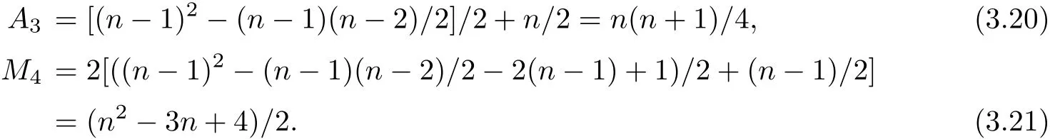
3.4.3Operation Counts in Total

Sum operation counts from(3.15)to(3.21)together,to evaluate Pn(xj)at N+1 points we require A additions and M multiplications,where

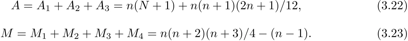
Now,we have a conclusion that to evaluate a polynomial of degree n at N+1 points with this new method,we drop n(N+1)multiplications of Horner’s method to n(n+2)(n+3)/4?(n?1) multiplications,although increase n(n+1)(2n+1)/12 additions in extra.Obviously,when N＞＞n,the multiplications and extra additions needed in our method could be negligible.For instance,given n=7,N=10000,we only require 0.217%multiplications and less than 0.1% extra additions comparing to the number of operations of Horner’s method.

3.5Numerical Experiments and Error Analysis

Computing performance and error analysis are done basing on several numerical experiments in both C language and Matlab.In this section,we will choose two typical experiments to demonstrate the advantage of our method.We computed P4(x)in Example 1,where

and P7(x),which is a Chebyshev polynomial,in Example 2,where

Both examples are computed by our method and Horner’s method respectively in Matlab. The results of P4(x)are plotted in the left subplot of Figure 1,while the results of P7(x)are plotted in the right subplot.As we can see in Figure 1,our method has a close accuracy with Horner’s method.If we consider the result of Horner’s method as exact result,the maximum absolute error of our method in Example 1 is 2.60206434177235×10?9and 3.20050941304828× 10?9in Example 2.Obviously,the accuracy of our method is acceptable for most of engineering problems.

Since Matlab is not a basic language,the execution time of program can not highly demonstrate the performance of our method,we compute Example 1 and Example 2 in C language. Given that Windows does not assign the same resource for every single execution of a program, we execute every program 500 times continuously and calculate the average executing time of a single execution.The result of this two examples are compared in Table 1.Obviously,the execution time of our method are far better than Honer’s method.

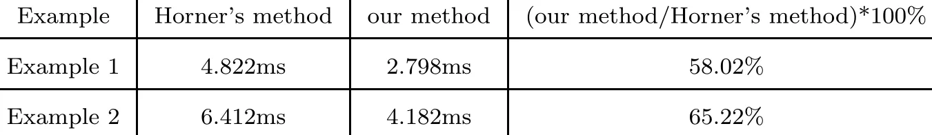
Table 1Comparison of Program Execution Time

Through the procedure and the results of Matlab implementations,we have found out:the maximum error point normally is the last entry of arithmetic progression.The error is mostly due to the recursive way we used in the procedure.As the roundof ferror of each recursion accumulates to the evaluation value,the maximum error probably exceed our tolerance whilewe have a large number of recursions,one solution for this problem is to divide the arithmetic progression into m new small arithmetic progressions.For each new arithmetic progression, we have L elements(L＞＞n).Evaluation values at the f i rst entry(xkL(k=1,2,···,m?1)) of these new arithmetic(exclude the f i rst one)are refreshed according to the method we use in Step 2.This refreshing gives more accurate values to P0,xL,P1,xL,P2,xL,···,Pn?1,xL.By properly choosing of m or L,we can achieve good performance in both accuracy and operation cost.

§4.Conclusions

In this paper,we have proposed a new fast method of polynomial evaluation at arithmetic progression.By using the recursive adding,we evaluated a polynomial of n degree at each entry of the arithmetic progression(not include the f i rst n entries)with only n additions,while no multiplication is required.Comparing with Horner’s method this method greatly saves computational ef f ort while N＞＞n of a polynomial.We have tested this method by several computational examples on Matlab and demonstrated its efficiency and accuracy.

[1]BOSTAN A,SCHOST′E.Polynomial evaluation and interpolation on special sets of points[J].Jornal of Complexity,2005,21(4):420-446.

[2]BORODIN A,MUNRO I.The Computational Complexity of Algebraic and Numeric Problems[M].New York:American Elsevier,1975.

[3]WINOGRAD S.On the number of multiplications necessary to compute certain functions[J].Communications on Pure and Applied Mathematics,1970,23(2):165-179.

[4]ELIA M,ROSENTHAL J,SCHIPANI D.Polynomial evaluation over f i nite f i elds:new algorithms and complexity bounds[J].Applicable Algebra in Engineering,Communication and Computing,2012,23(3-4): 129-141.

[5]ABBAS M,GUSTAFSSON O.Computational and Implementation Complexity of Polynomial Evaluation Schemes[C].Lund:NORCHIP,2011:1-6.

[6]REY NOLDS G S.Investigation of Dif f erent Methods of Fast Polynomial Evaluation[D].Edinburgh:University of Edinburgh,2010:7-18.

tion:65Y04,68M07

1002–0462(2014)04–0509–07

date:2012-12-24

Supported by the Graduate Starting Seed Fund of Northwestern Polytechnical University(Z2012030)

Biographies:LU Jiang-kang(1956-),male,native of Xi’an,Shaanxi,an associate professor of Northwestern Polytechnical University,M.S.D.,engages in advanced technology of electrical engineering;CHEN Haibiao(1985-),male,native of Chaozhou,Guangdong,M.S.D.,engages in computational electromagnetic;JING Rui-xing(1987-),female,native of Zhengzhou,Henan,M.S.D.,engages in advanced technology of electrical engineering.

CLC number:O241.81Document code:A