
Bethe ansatz solutions of the 1D extended Hubbard-model
2024-05-09 05:19:22HaiyangHou侯海洋PeiSun孫佩YiQiao喬藝XiaotianXu許小甜XinZhang張鑫andTaoYang楊濤
Haiyang Hou (侯海洋) ,Pei Sun (孫佩),2 ,Yi Qiao (喬藝),2 ,Xiaotian Xu (許小甜),2,? ,Xin Zhang (張鑫) and Tao Yang (楊濤),2
1 Institute of Modern Physics,Northwest University,Xian 710127,China
2 Shaanxi Key Laboratory for Theoretical Physics Frontiers,Xian 710127,China
3 Beijing National Laboratory for Condensed Matter Institute of Physics,Chinese Academy of Sciences,Beijing 100190,China
Abstract We construct an integrable 1D extended Hubbard model within the framework of the quantum inverse scattering method.With the help of the nested algebraic Bethe ansatz method,the eigenvalue Hamiltonian problem is solved by a set of Bethe ansatz equations,whose solutions are supposed to give the correct energy spectrum.
Keywords: quantum integrable system,Bethe ansatz,T-Q relation,Hubbard model
1.Introduction
The 1D Hubbard model [1] is one of the most important solvable models in non-perturbative quantum field theory[2].It exhibits on-site Coulomb interaction and correlated hopping,which helps us to understand the mystery of high-Tcsuperconductivity.It is a paradigm of integrability in the strongly correlated systems.
In the past several decades,numerous approaches have been proposed to study the integrability and the physical properties of the 1D Hubbard model [3–12].The Hubbard model with a periodic boundary condition was first exactly solved via the coordinate Bethe ansatz method [13,14].Shastry then constructed the correspondingR-matrix and the Lax matrix,and demonstrated the integrability of the 1D Hubbard model [15,16].The Hamiltonian of the conventional Hubbard model can be constructed by taking the derivation of the logarithm of the quantum transfer matrix atu=0,{θm=0}.Martins and his co-workers subsequently gave the solution of the conventional Hubbard model via the nested algebraic Bethe ansatz approach [17].
Our starting point is the construction of an extended 1D Hubbard model.We let all the inhomogeneous {θm} in the transfer matrix take the same nonzero value θ,i.e.u=θ,{θm=θ}.Then,the derivative of the logarithm of the quantum transfer matrixt(u) atu=θ gives another integrable Hamiltonian.This model depends on more free parameters.Compared to the conventional Hubbard model,the new model contains more possible nearest-neighbor interactions.Following the nested algebraic Bethe ansatz method,we solve the extended Hubbard model exactly.TheT-Qrelation and a set of Bethe ansatz equations (BAEs)are proposed.
This paper is organized as follows.In section 2,we construct an integrable 1D extended Hubbard model.In section 3,we formulate the nested algebraic Bethe ansatz for the extended Hubbard model and present our main results.Section 4 is devoted to the conclusion.
2.1D extended Hubbard model
Let us recall the formulation of the integrability of the 1D Hubbard model [16].The quantumR-matrix is given by [15],
where,
and functionsh1≡h(u),h2≡h(v) are assumed to satisfy the constraint:
Wadati proved that theR-matrix in (1) indeed satisfies the Yang–Baxter equation [18]:
We construct the monodromy matrix:
where {θ1,…,θN} are inhomogeneous parameters.T0(u) in equation (5) satisfies the RTT relation:
The transfer matrix is thus:
which has the commutative property:
In the homogeneous limit {θm=θ},the derivation of the logarithm of the transfer matrix atu=θ gives the following Hamiltonian:
From the constraint in (3),one can obviously see that the functionh(θ) is determined by θ andU.Therefore,the Hamiltonian depends on two independent parameters θ andU.The Hermitian condition of the Hamiltonian reads as follows:
Moreover,in order to relate the coupled spin model in(9)to the Hubbard model,we have to perform the following inverse Jordan–Wigner transformation:
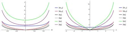
Figure 1. Left: interaction intensity |αk| versus θ/i with U=2.5.Right: interaction intensity |αk| versus U with θ=0.5i.
where the parameters {α1,…,α8} are given by,
The Hamiltonian (12) contains most of the possible nearest-neighbor interactions appearing in strongly correlated systems,e.g.the kinetic energy possessed by particles,the hopping terms that are also included in the conventional Hubbard model,the spin-spin interaction that is the familiar spin-exchange term of the Heisenberg XXX spin chain,and the pair hopping term that relates to the simultaneous hopping of two electrons from one site to a neighboring site.
The interaction intensities {α1,…,α8} all depend on θ andU.For finite θ andU,they are all of the same order of strength,which is clearly illustrated in figure 1.
Compared to Alcaraz’s model [11],whose integrability has not been proved,the model we construct is integrable and Hermitian.Shiroishi presented two integrable Hamiltonians[19] that only depend on one free parameter.While,in this paper,we use a differentR-matrix and construct a more general integrable Hamiltonian related to two free parameters θ andU.
The new Hamiltonian in(12)reduces to the conventional Hubbard model at θ=0,namely:
In conclusion,we construct a more general integrable Hamiltonian via the quantum inverse scattering method(QISM).
3.Exact diagonalization of the transfer matrix
In this section,we expect to diagonalize the transfer matrix and obtain the corresponding Bethe ansatz equations by following the procedure of the nested algebraic Bethe ansatz method [17,20,22].We first represent the monodromy matrix (5) in the matrix form:
The transfer matrix can be expressed by,
We introduce the local vacuum state at sitej:
Then,the global vacuum is constructed as,
The elements of the monodromy matrixT0(u) have the following effect on the reference state |0〉:
One can see that the total number of particles is conserved andBk(θ)is a creation operator.The eigenstate oft(u)can thus take the form:
where {λ1,…,λM} is a set of Bethe roots and the repeated indices indicates the sum over the values 1 and 2,andare certain functions of {λj}.
Before we go any further,let us introduce the following useful commutation relations:
which can be derived from the RTT relation (6).Here,the superscript represents the row and the subscript represents the column.The matrixr(u,v) in (23) is defined as,
with,
Using the commutation relations (23),we have:
where u.t.denotes the unwanted terms andPis the permutation operator.Here,t(1)(u,{λj}) is the nested transfer matrix:
where,
Applying the transfer matrixt(u) to the state |λ1,…,λM〉 and using the commutation relations (21)-(23) repeatedly,we obtain:
where Λ(1)(u,{λj}) is the eigenvalue oft(1)(u,{λj}) in (27).
The function Λ(1)(u,{λj}) can be given by the algebraic Bethe ansatz method [22]:
wherem=0,…,Mand {μ1,…,μm} are the second set of Bethe roots.
Define the following functions:
Then,we can easily check the following useful relations:
Substituting equation (30) into equation (29),the eigenvalue Λ(u) of the transfer matrixt(u) (7) can be parameterized as,
whereM,m?N and 0≤m≤M≤2N.
We introduce the following short-hand notations:
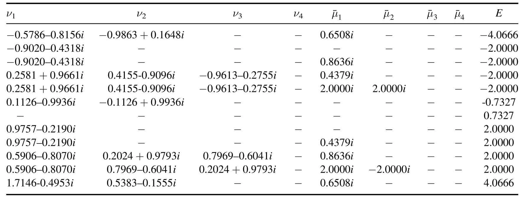
Table 1. The numerical solutions of the BAEs (37) and (38) for N=2,θj=θ=0.17i and U=1.3.The energy E calculated from equation (40) are the same as those from the exact diagonalization of the Hamiltonian.
and
Thus,the eigenvalue Λ(u)in(33)can be rewritten in a simpler form:
To eliminate the unwanted terms in equation (29),the Bethe roots {λ1,…,λM} and {μ1,…,μm} should satisfy two sets of BAEs:
where,
The eigenvalue of the Hamiltonian (9) in terms of the Bethe roots is:
The numerical solutions of the BAEs (37) and (38) for theN=2 case are shown in table 1.The energy spectrum given by Bethe roots is consistent with the ones from the exact diagonalization of the Hamiltonian.
When θ=0,our extended Hubbard model degenerates into the conventional one.As a consequence,the corresponding BAEs and the eigenvalue of the Hamiltonian reduce to,
4.Conclusion
In this paper,we study a 1D extended Hubbard model with a periodic boundary condition.We construct an integrable Hamiltonian (12) within the framework of the QISM.Compared with the conventional Hubbard model,the extended one contains more interaction terms.Using the nested algebraic Bethe ansatz method,the eigenvalue problem of the extended Hubbard model is solved by the homogeneousT-Qrelation(36) and the associated BAEs (37) and (38).The numerical simulations imply that the solutions of the BAEs (37) and(38) indeed give the correct spectrum of the Hamiltonian.It should be noted that theT-Qrelation (36) and BAEs (37)and (38) are constructed by selecting an all spin-up state as the vacuum state and they may not give the complete solutions.There also exists anotherT-Qrelation with an all spin-down state being the vacuum.These two Bethe ansatz should give the complete set of eigenvalues and eigenstates of the Hamiltonian.
Furthermore,one can study the explicit form of the eigenstate in equation (20).In addition,based on our homogeneous BAEs,the thermodynamic properties of the model can also be studied via the well-known thermodynamic Bethe ansatz method [21].
Another interesting objective is to construct integrable extended Hubbard models with open boundary conditions.These models can be exactly solved via the off-diagonal Bethe ansatz method[22].For open systems,we can study the thermodynamic limit of the model through the novelt-Wscheme [23,24].
Acknowledgments
Financial support from the National Natural Science Foundation of China(Grant Nos.12105221,12175180,12074410,12047502,11934015,11975183,11947301,11775177,11775178 and 11774397),the Strategic Priority Research Program of the Chinese Academy of Sciences (Grant No.XDB33000000),the Shaanxi Fundamental Science Research Project for Mathematics and Physics (Grant No.22JSZ005),the Major Basic Research Program of Natural Science of Shaanxi Province (Grant Nos.2021JCW-19,2017KCT-12 and 2017ZDJC-32),the Scientific Research Program Funded by the Shaanxi Provincial Education Department (Grant No.21JK0946),the Beijing National Laboratory for Condensed Matter Physics (Grant No.202162100001) and the Double First-Class University Construction Project of Northwest University is gratefully acknowledged.
ORCID iDs
猜你喜歡
Plasma Science and Technology(2022年5期)2022-06-01 07:55:38
當(dāng)代黨員(2022年9期)2022-05-20 13:35:21
當(dāng)代黨員(2022年9期)2022-05-20 13:35:21
初中生學(xué)習(xí)指導(dǎo)·中考版(2022年4期)2022-05-12 00:12:51
Chinese Physics B(2022年4期)2022-04-12 03:47:22
Chinese Physics B(2021年5期)2021-05-24 02:24:48
Acta Mathematica Scientia(English Series)(2020年6期)2021-01-07 06:44:22
當(dāng)代音樂(2018年4期)2018-05-14 06:47:13
琴童(2017年7期)2017-07-31 18:33:48
小學(xué)科學(xué)(2017年5期)2017-05-26 18:25:53
 Communications in Theoretical Physics2024年4期
- Communications in Theoretical Physics的其它文章
- Exploring dielectric phenomena in sulflowerlike nanostructures via Monte Carlo technique
- Electrical characteristics of a fractionalorder 3 × n Fan network
- Theoretical study of the nonlinear forceloading control in single-molecule stretching experiments
- Diffusion of nanochannel-confined knot along a tensioned polymer*
- Two-component dimers of ultracold atoms with center-of-mass-momentum dependent interactions
- Phase structures and critical behavior of rational non-linear electrodynamics Anti de Sitter black holes in Rastall gravity