
A deep learning method based on prior knowledge with dual training for solving FPK equation
2024-01-25 07:11:34DenghuiPeng彭登輝ShenlongWang王神龍andYuanchenHuang黃元辰
Chinese Physics B 2024年1期
關(guān)鍵詞:神龍
Denghui Peng(彭登輝), Shenlong Wang(王神龍), and Yuanchen Huang(黃元辰)
School of Mechanical Engineering,University of Shanghai for Science and Technology,Shanghai 200093,China
Keywords: deep learning,prior knowledge,FPK equation,probability density function
1.Introduction
The Fokker–Planck–Kolmogorov (FPK) equation governs the temporal evolution of probability density functions(PDFs) within a stochastic dynamic system, which stands as one of the foundational equations for investigating stochastic phenomena.The FPK equation is widely utilized in many fields, such as biology,[1]chemistry,[2]economics,[3]applied mathematics,[4]statistical physics,[5]and engineering.[6]By integrating the PDF of the stochastic dynamic system,one can obtain the probability distribution and mathematic expectation of macroscopic variables.When the excitation of the stochastic dynamic system is Gaussian white noise,the corresponding FPK equation is one type of the second-order parabolic partial differential equation(PDE),whose analytical solution can be obtained only in some particular cases.Therefore,in most cases,the numerical method is considered feasible to solve the FPK equation.
In the past few decades, a large number of numerical methods based on meshing have been used to solve the FPK equation, such as the finite element method,[7]finite difference method,[8]path integration method,[9]and variation method.[10]The disadvantage of the above methods is that they can only be solved at grid points, and the solution at any points other than grid points requires reconstruction or interpolation.Moreover, for high-dimensional systems, the dependence of those methods on grid division leads to a sharp increase in the amount of data, and the solution procedure would be quite time- and resource-consuming.In addition,Monte Carlo simulation(MCS)is also frequently employed to address the FPK equation,[11]which approximates the probability density distribution either by sampling extended trajectories of the stochastic differential equation(SDE)or through the application of the conditional Gaussian framework.[12]The correctness of the solution for this method depends on the volume of data collected,despite the fact that it does not require interpolation.Furthermore, for high-dimensional systems, it can be barely possible to obtain the joint probability density function (JPDF) of high accuracy using the aforementioned approaches due to the large computational cost involved.
Recently, the increasing abundance of computing resources and the rapid development of neural networks (NNs)has provided a promising way to solve the PDEs.[13–17]For general high-dimensional parabolic PDEs, Hanet al.[13]designed a deep learning (DL) framework which used backward SDEs to reformulate PDEs and used NNs to approximate the gradient of solutions.Raissiet al.[14]proposed a DL method to solve the forward-backwards SDEs and their corresponding high-dimensional PDEs.Subsequently, they proposed physics-informed neural network(PINN)by embedding physical information into the NN.[15]The method could be applied to a wide range of classical problems in fluids and quantum mechanics.Berget al.[16]used deep feedforward artificial NNs to approximate the solution of PDEs in complex geometry and emphasized the advantages of the deep NN compared with the shallow one.Sirignanoet al.[17]were dedicated to solving higher-dimensional PDEs using a deep Galerkin method which trained the NN to meet the differential operator form, initial and boundary conditions.Despite the fact that the FPK equation is a PDE, the methods mentioned above cannot be used to solve the FPK equation.The primary cause is that the equation format lacks a constant term and there is no probability distribution at the boundary,which make that zero is used as a trial solution.Consequently, numerous methods for solving FPK equation based on DL have been proposed.[18–27]Among them, Xuet al.[18]proposed a method for solving general Fokker–Planck (FP) equations based on DL called DL-FP, which innovatively added normalization conditions and set penalty factors in the supervision conditions to avoid zero trial solution and skip local optima.However, the normalization condition of this method is closely related to global information,which means that the calculation data will grow exponentially with the increase of dimension, and the method will thus fall into the curse of dimension when solving higher-dimension problems.Subsequently, Zhanget al.[19]optimized the training data on the basis of DL-FP.A suitable and small number of discrete integral points and integral volumes were obtained through multiplek-dimensional-tree(KD-tree)segmentation of the random data set, which solved the problem brought by the global information that needs to be considered.Furthermore, they designed a new DL framework that included multiple NNs and matched one NN for each dimension,making the training data grow linearly instead of exponentially.[20]Wanget al.[21]proposed an iterative selection strategy of Gaussian neurons for radial basis function neural networks (RBFNN) which is applied to obtain the steady-state solution of the FPK equation.The strategy is much more efficient than the RBFNN method with uniformly distributed neurons.Another approach is to use the PDF calculated from prior data to supervise the solution of the FPK equation instead of the supervision of the normalization condition.[22,23]Among them,Zhaiet al.[23]developed a meshless FPK solver that used prior data from the solution of the FPK equation obtained from MCS as a supervised condition instead of a normalized condition, which not only excluded zero solution but also avoided data explosion.Nevertheless, that method still needs improvement, since the prior data supervising the solution obtained from numerical simulations is relatively rough.
In general, the speed and accuracy of the above methods are not always guaranteed.For the DL-FP method,[18]the presence of normalization conditions in the loss function makes the solution less efficient and less applicable.For meshfree methods,[23]it is a good idea to utilize prior knowledge to guide the solution process to avoid normalization conditions.However, it is not a suitable choice to use prior knowledge containing gradient information errors together with the FPK differential operator to guide the solution process, even if the NN is robust.Inspired by the above methods,we propose a DL method based on prior knowledge(DL-BPK)to solve the FPK equation.The proposed method is composed of dual training processes: the pre-training process and the routine training or prediction process.In pre-training, the prior knowledge obtained from MCS is injected into the training to obtain a pretrained model.The role of the pre-trained model is to make the NN jump out of the local optimum faster to accelerate the training process, especially in high dimension, which is similar to the function of initializing network parameters.Based on the pre-trained model,the FPK differential operator is used as a supervised condition to make the final solution sufficiently smooth and accurate.In addition to the FPK differential operator,a supervised condition should be set to suppress the generation of zero solutions.Herein, the points with the highest probability density within a small range under the pre-trained model, which is the local maximum point, will be selected as the supervision points.There are two reasons for this setting: one is to avoid generating zero trial solution, and the other is to minimize perturbations in the shaping of the PDF,attributable to the absence of gradient information errors.Finally,the PDF generated by the NN undergoes normalization,a process that serves to correct errors in the PDF value.In summary,the main contributions of this article are as follows: (i)Introducing a new supervised condition based on local maximum points and FPK differential operator forms,significantly improving the accuracy and robustness of the solution;(ii)The implementation of pre-trained models based on prior knowledge reduces training costs and accelerates the convergence of NNs.
The rest of this article is organized as follows: the DLBPK method is detailly described in Section 2.In Section 3,we use four examples to verify the effectiveness of our method.These examples include two two-dimensional (2D)systems, one six-dimensional (6D) system, and one eightdimensional(8D)system.At the same time,the comparisons between the proposed method and the analytical solution, as well as other methods, are carried out to demonstrate the superiority of the proposed method.In Section 4, the impact of the pre-trained model and penalty factors on the results are discussed.Finally,Section 5 presents conclusions to close this paper.
2.Methodology
In this section, the FPK equation and the necessary conditions for its solution are described in detail in Subsection 2.1 and a detailed introduction to the DL-BPK method is then provided in Subsection 2.2.
2.1.The FPK equation
Consider the general form of SDEs
whereX=[x1,...,xi,...,xn]Tdenotes ann-dimensional variable,f(X) represents ann-dimensional vector function ofX,σ(X)serves as a square matrix that is assumed to be constant later in the paper andW(t)is ann-dimensional standard Gaussian white noise.For Eq.(1),the probability density distribution thatXobeys is described by its corresponding FPK equation
whereLFPKis the FPK differential operator,andp(X),the solution of the FPK equation,denotes the PDF of the stochastic processX.Here, this paper studies the stationary FPK equation with natural boundary,which takes the following form:
Moreover,the boundary conditions should be satisfied
Then, the normalization condition should be preserved for PDF
Combining Eqs.(2)and(3),it can be seen that the stationary FPK equation is a type of the second-order PDE.There is no constant term in the equation, which means that zero will become its trial solution.In short, the solution of FPK equation should bear the following four characteristics: (i)it must conform to the form of FPK equation;(ii)the probability density at the boundary is 0; (iii)as a PDF,normalization should be considered;(iv)it should be nonnegative.
2.2.The algorithm
Before describing the proposed method, two existing methods to solve the FPK equation are first introduced.The method proposed in Ref.[18] sets the discretization form of Eqs.(3)–(5)as three supervised conditions in the loss function of the NN, and introduces a penalty factor.The form of the loss function is as follows:
wherepθ(·) represents the trial solution of the FPK equation obtained by NN,θbeing the parameters of the NN, which will be updated continuously during training of the NN.The second term in Eq.(6)is the integral approximation of all the uniformly discrete points in the region to satisfy the normalization condition.It indicates that the number of the calculation points increases exponentially with the increase of dimensionality,which leads to considerable growth in computational cost,and makes the application of this method in highdimensions almost impractical.In addition, the redundancy of supervised conditions inevitably makes the NN easy to fall into local optima, and even unable to converge after a long time.Even though the penalty factor alleviates this problem to some extent,the effect is not ideal.It is still necessary to find an approach to make the NN skip the turbulence in the early training stage and accelerate the fitting.
Another method to solve the FPK equation is using the PDF calculated from prior data instead of the normalized condition to supervise the solution of FPK equation.[23]The associated loss function is given by
where ?p(·)is an approximate estimate of the probability density,as determined by MCS.The second term in Eq.(7)serves to replace both the normalization and boundary conditions.This suggests that the exclusive use ofNytraining points with probability density, as opposed to using a large number of points for normalization,can yield superior guidance for PDF generation.As a result, it effectively mitigates the challenge of data explosion encountered in high-dimensional cases.Although the presence of the FPK operator has been demonstrated to confer robustness to NNs and facilitate the use of rough prior knowledge in approximating FPK equation solutions, such prior knowledge can still pose challenges for NN training.Specifically,it can complicate the initial training process and potentially limit the accuracy of the final solution.
To address this problem, a pre-trained model is introduced to prevent the difficulty of fitting NNs.Meanwhile,the normalization condition is replaced by newly added supervision conditions to avoid zero trial solution.The detailed procedures of the DL-BPK method for solving FPK equation are described below,and the flow chart is shown in Fig.1.
Step 1 Constructing the training set
Due to the limited training set of NNs, MCS is utilized to obtain the range of variables in each dimension, and the range is defined as the bounded domain?.Each dimension of?is then discretized by step length Δx.For thendimensional case, the range of its variables in each dimension is assumed to be [a,b]n, and the number of training data and that of boundary data areND=((b?a)/Δx)nandNB=2n((b?a)/Δx)n?1, respectively.As a result, the training set becomesTD=XDi ∈?NDi=1, which consists of uniformly spaced grid points covering?; the boundary set isTB=XBi ∈??NBi=1, which represents the boundary of the training set.Subsequently, we adopt the Euler–Maruyama method to generate a long trajectory for Eq.(1), and selectNSpoints to form a training setTS=XSi ∈?NSi=1.The probability density of this training data can be obtained from MCS simulation.The training setTSand ?p(TS) are used as prior knowledge to pretrain the NNs.An important clarification is that the MCS used to generate prior knowledge in this study were run on small sample sizes.Although this approach comes at the expense of the accuracy of the a priori knowledge obtained,it does speed up the collection of data.
Step 2 Training the NNs
Setting the loss function as follows:
Similar to Eq.(6),pθ(·)is employed to denote the PDF solution obtained from the NN.To differentiate the results from the dual-training stages of the DL-BPK method,we usepθ1(·)andpθ2(·)for the PDF solutions after the first and second rounds of training,respectively.In the method proposed in this paper,the NNs need pre-training to prevent the difficulties in fitting during the actual training process.L1should be minimized to ensure that the obtained pretrained model can generate the distribution of prior knowledge,and MCS is applied to get the PDF of prior data.
In addition, in the actual training process,L1in Eq.(8)can be reduced to a satisfactory value with only thousands of iterations, which is due to the simplicity of the loss function term and the small amount of data.It should be noted that the time cost for obtaining the pre-trained model is small.The accuracy of the solution of the pre-trained model still needs improvement, so further training is performed.In this training,LFPKis considered as a supervision condition, and it is also necessary to constrain it to prevent the generation of zero solutions.The loss function for this further training is defined as follows:
wherepθ1(XLi) is the probability density of the pretrained model atXLi, and the data setTLincludesNLpoints sampled from the local maximum points of PDF of the pre-trained model (NL=1 for a general monostable distributed system).It can be seen from Eqs.(10) and (11) thatE1ensures the final solution is in the FPK form, andE2supervises the solution of the FPK equation using the PDF calculated at local maximum points by the pre-trained model.The main purpose ofE2is to exclude zero solution.The local maximum points are selected to avoid introduction of spatially related gradient noise information.It should be noted that although the NN has good robustness,elimination of noise information greatly facilitatesE1training and enhances the accuracy of training results.In summary,the pretrained model is designed to provide more suitable initial parameters for subsequent training,which plays a significant role in the fast fitting of NNs,especially when solving high-dimensional problems.In addition,sinceL2does not include a loss function term with spatial gradient noise information, the accuracy of the final solution is satisfactory,as to be shown in Section 3.
Step 3 Setting the parameters of the NN
In this paper,the Adam optimizer is used to minimizeL1andL2.Unless otherwise specified, the NNs all have 4 hidden layers and 20 hidden nodes.To guarantee both the nonnegativity and differentiability of the PDF output generated by the NN, the sigmoid function is employed as the activation function.In Eq.(9),the FPK form controls the smoothness of the solution, which directly affects the accuracy of the solution.Therefore, we are more interested in the decline ofE1.In this regard,the penalty factorλis designed to influence the process of supervised training,and to reduce the weight ofE2,so that the NN approaches the shape of the exact solution.It should be pointed out that due to the reduction ofE2weight and the rough probability density of the local maximum point,the final solution cannot well satisfy the normalization conditions.In order to make the final result standardized,the Vegas integral technology[28]is used to complete the normalization.
3.Examples
In this section, four numerical examples are provided to support our conjecture,and to prove that DL-BPK method can be used successfully.In the first example, we showcase the advantages of DL-BPK over other deep learning methods in terms of both speed and accuracy, while also examining the influence of the number and type of supervision points on the results.The second example considers a 2D steady-state toggle switch system,using MCS results to demonstrate the suitability of DL-BPK.The third and fourth examples further illustrate the applicability of the method to high-dimensional systems.
3.1.A two-dimensional stochastic gradient system
Considering a 2D stochastic gradient system[23]
whereΓ1andΓ2are independent standard Gaussian white noise excitation with zero mean-value andσdenotes the noise intensity.Then lettingV=V(xy)=(x2+y2?1)2and the reduced stationary FPK equation is
and the precise steady-state solution can be expressed as
whereCbeing the normalized constant.In this example, the selected calculation area is?=[?2,2]2and the system parameterσ=1.
Utilizing the DL-BPK method, we set Δx=0.04, so the training setTDcomprised 104data,while the boundary setTBencompassed 400 data.For the system(12),TSwas acquired by selecting 104training data from the trajectory obtained by running the Euler–Maruyama numerical method with 108steps.The probability density ofTScan be obtained through MCS and the penalty factor is set toλ=0.01.The DL-BPK method is then employed to solve Eq.(13) according to the steps described in Subsection 2.2.The pretrained model is obtained after 2000 iterations of the NN, and the training set as well as the loss function were updated and further trained 4×4times to get the final result as shown in Fig.2.The DLBPK solution closely mirrors the exact solution determined by Eq.(14), with a maximum absolute error in the JPDF of approximately 1.4×10?4.Figure 2(f)shows the comparison of the exact solution and the DL-BPK solution for marginal probability density function (mPDF) ofp(x), wherep(y) is identical.Visually,the outcomes are practically indiscernible.In addition,by comparing the results of DL-BPK and the pretrained model, it can be seen thatLFPKgreatly improve the accuracy and smoothness of the solution.It is also proved that the accuracy of the DL-BPK solution would not be affected by the pre-trained model.The result of the pre-trained model is not satisfactory, but its accuracy is not the focus of our research.The function of the pre-trained model is more embodied in accelerating NN fitting.Moreover, it should be mentioned that in this example,we selected 4 uniformly sampled local maxima of the PDF of the circular distribution of the pre-trained model as the supervision points.
In order to illustrate the advantages of the pre-training and to demonstrate the superiority of the DL-BPK method in training speed, we tested DL-BPK, DL-FP[18]and the mesh-free data-driven solver[23]simultaneously to solve system(12).In order to assess and measure the effectiveness and accuracy of the proposed method,we defined
wherepsbeing the exact solution,and‖·‖2denoting theL2norm.The closerRaccis to 1,the higher the result accuracy is.This test used data set of the same size and ran on the same device.The experimental conditions and parameter settings are shown in Table 1,in which the optimizer defaults to Adam and the learning rate automatically adjusts with the number of iterations,and the obtained results are shown in Fig.3.
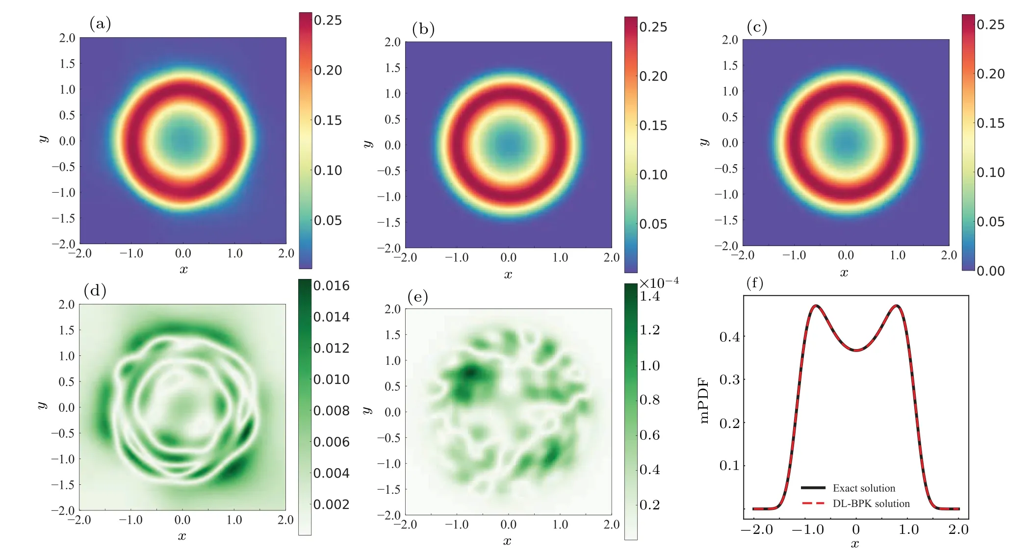
Fig.2.Results for system(12): (a)solution of pre-trained model;(b)solution of DL-BPK;(c)exact solution;(d)solution error of pre-trained model;(e)solution error of DL-BPK;(f)contrast of solution for one-dimensional(1D)mPDF.
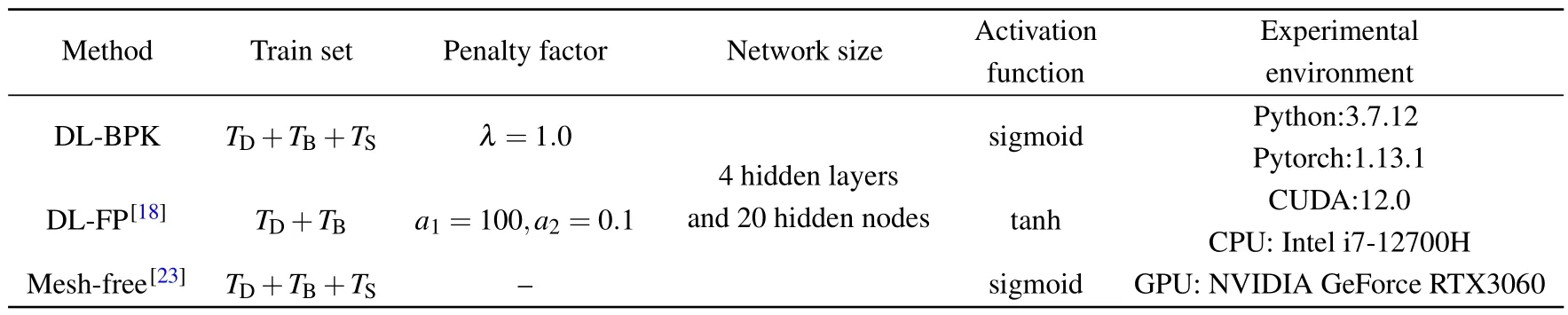
Table 1.Experimental environment and parameter settings.
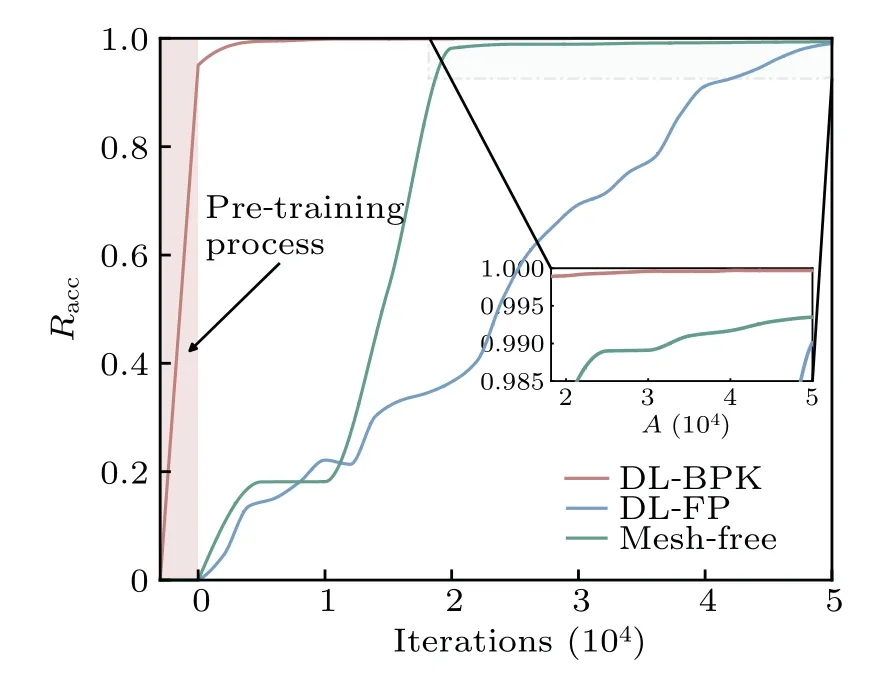
Fig.3.Comparison of results from different methods.
It is clearly observed that the NN can be fitted more quickly after pre-training.Compared to other methods, the proposed DL-BPK method achieves the same accuracy with fewer iterations: an accuracy of over 99.8% in less than 420 seconds (including pre-training).It can also be seen through local zooming in Fig.3 that the final accuracy of DL-BPK is very high, reaching around 99.97%.Additionally, figure 3 also shows that other deep learning methods may fall into fluctuations in the early stage of training, which requires a lot of time to get rid of.It further validates the importance of pretraining.Furthermore, we will discuss in detail the effect of errors of pre-trained PDF on the final PDF in terms of convergence speed and ultimate error in Subsection 4.1.
In addition,the advantage of using local maximum points as the supervision points are verified using this example.To this end, 4, 20, 100, and 400 local maximum points are obtained from the prior distribution as supervision points, and then 4, 20, 100, and 400 points are randomly selected from the trajectory of the system (12) as supervision points.Their probability density is obtained from the exact solution with artificially injected noise,rather than from the pre-trained model.The purpose is to study the performance of the solution with rough supervision points, by adjusting the magnitude of the noise intensity,which simulated the actual solving process using inaccurate information.Specifically, we obtain a set of supervision pointsTLand calculateps(XLi), thenpθ1(XLi)=(1?ε+2εU)·ps(XLi), whereUis uniformly distributed on[0, 1].The maximal relative errorεof noise is set to 0, 0.1,0.3,0.5,and 0.8,respectively.It should be noted that this test is trained 104times on the basis of the pre-trained model to ensure that the NN basically fit.The results are shown in Fig.4.
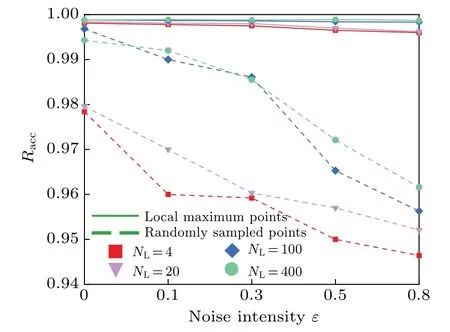
Fig.4.Accuracy under different numbers and types of supervision points and different noise intensities.
It is evident that using local maximum points as supervision points mitigates the impact of increased noise intensity on result accuracy.In contrast, when supervision points are randomly sampled, accuracy tends to decline as noise intensity rises.This phenomenon can be attributed to two factors:First,the probability density at randomly sampled supervision points varies significantly,exacerbating the gradient information error between them when noise is high,thereby affecting the minimization ofE1.Second, when the supervision point corresponds to a local maximum in the PDF,any inaccuracies in its value are offset during the final normalization process.Finally, it is worth noting that increasing the number of supervision points, whether they are local maximum points or randomly sampled points from the trajectory,improves adaptability to roughness.However, to minimize the reliance on prior knowledge,the preference is to select a smaller number of supervision points.
3.2.A 2D multi-stable toggle switch system
It is challenging to solve multi-stable systems with low noise, and we would like to test the performance of the DLBPK method in such special situations.Considering a toggle switch system[29]
whereΓ1andΓ2are the independent standard Gaussian white noise excitation with zero mean-value andσdenotes the noise intensity.The reduced stationary FPK equation is
For this system, the selected calculation area is?=[0,1.5]2and constantb=0.25.We set Δx=0.015, so the training setTDcomprised 104data,while the boundary setTBencompassed 400 data.For Eq.(15),TSwas acquired by selecting 104training data from the MCS simulation with 105steps and the penalty factor is set to 0.001.For Eq.(16), the results of DL-BPK method on JPDF are shown in Fig.5.In addition,similar to the above example,the DL-FP,mesh-free,and DLBPK method proposed in this paper are tested on this example.It should be noted that this system does not have an analytical solution,so we will compare the results of 108steps simulated using MCS, which took 1.5 hours, and the final results and comparison are shown in Fig.6.
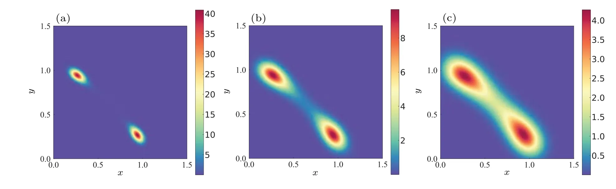
Fig.5.The DL-BPK solution of system(15)with different noise intensities: (a)σ =0.05,(b)σ =0.1,(c)σ =0.15.
From Figs.5 and 6, the results clearly indicate that finding a solution becomes more challenging when the noise intensity is low.However, the DL-BPK method still maintains good performance in less than 500 seconds (including pretraining).This is attributed to the adaptability of the method when local maximum points are used as supervision points,even in the presence of rough prior knowledge distributions.This has been proven in system (12).As the noise intensity increases, the performance of the Mesh-free method also improves,likely due to the increased accuracy of the prior knowledge.As for the DL-FP method, its inability to capture the distribution characteristics of the system even after more than 3×10⁴iterations highlights the particular challenges posed by this system.This also underscores the significant advantages of using prior knowledge when solving complex systems.
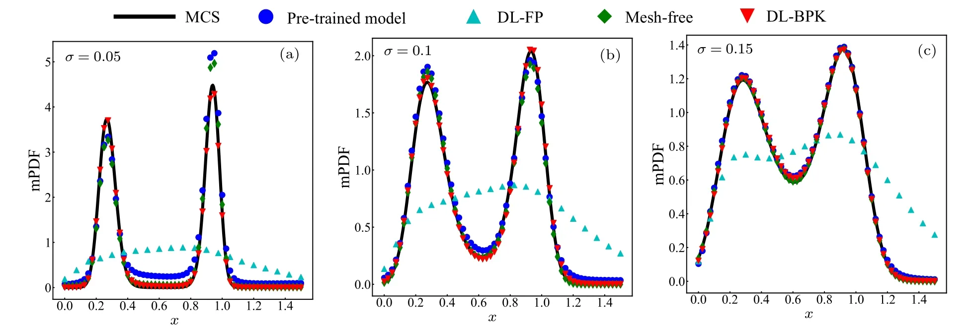
Fig.6.Comparison of results of different methods for mPDF p(x)under three different incentives.
For bistable distribution systems with low noise intensity,the accuracy of the distribution is compromised when fewer MCS simulations are used to obtain prior knowledge.The inaccuracy subsequently affects the distribution of the pretrained model and the probability density of the supervision points,thereby slightly impacting the final results.We anticipate addressing this issue through improved sampling methods in future work.It is worth noting that there have been studies focused on solving low-noise systems.[24]Additionally,the test yielded optimal results when the number of hidden nodes was set to 50,aligning with observations in system(15).This suggests that wider NNs are more effective at approximating highly concentrated probability distributions compared to their narrower counterparts.
3.3.A 6D system
Consider a 6D system[19]
wherein,Γi(wherei= 1, 2, 3) denotes independent standard Gaussian white noise excitation with zero mean-value andσi(wherei=1, 2, 3) denotes the noise intensity.AndThe corresponding stationary FPK equation is
whereCbeing the normalization constant.For this system,the range of training set is set to[?5,5]6,and there are 5.0×10⁵data in the training setTD, and 1.5×10⁵data in the boundary setTB.1.0×105points are sampled from the trajectory of the system (17) to formTS.The probability density ofTScan be obtained through MCS and the penalty factor is set toλ=0.01.The pre-training is carried out 5000 times and then the actual training 5×10⁴times to obtain the final solution.The results of Eq.(18)are shown in Fig.7.By comparing the final solution with Eq.(19), which is the exact solution, the DL-BPK method still performs well in terms of accuracy on the six dimensions.
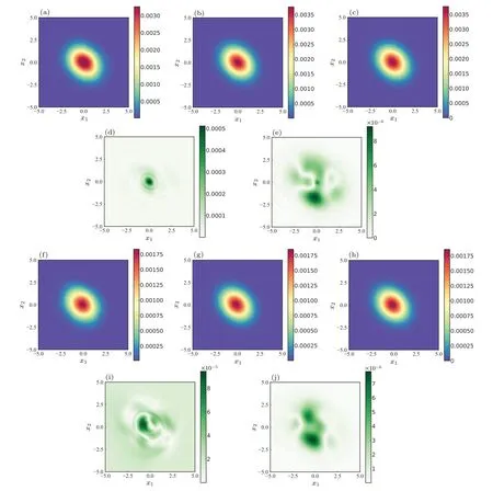
Fig.7.Results for system(17)with σ21 =σ22 =σ23 =2.0.Comparing probability densities on central slices in 6D state space: (a) p(x1,x2|y1=y2=x3=y3=0)of pre-trained model;(b) p(x1,x2|y1=y2=x3=y3=0)of DL-BPK method;(c)analytical p(x1,x2|y1=y2=x3=y3=0);(d)solution error of panel(a);(e)solution error of panel(b).Similarly,panels(f)–(j)are solutions for p(x1,x2|others are 0.6).
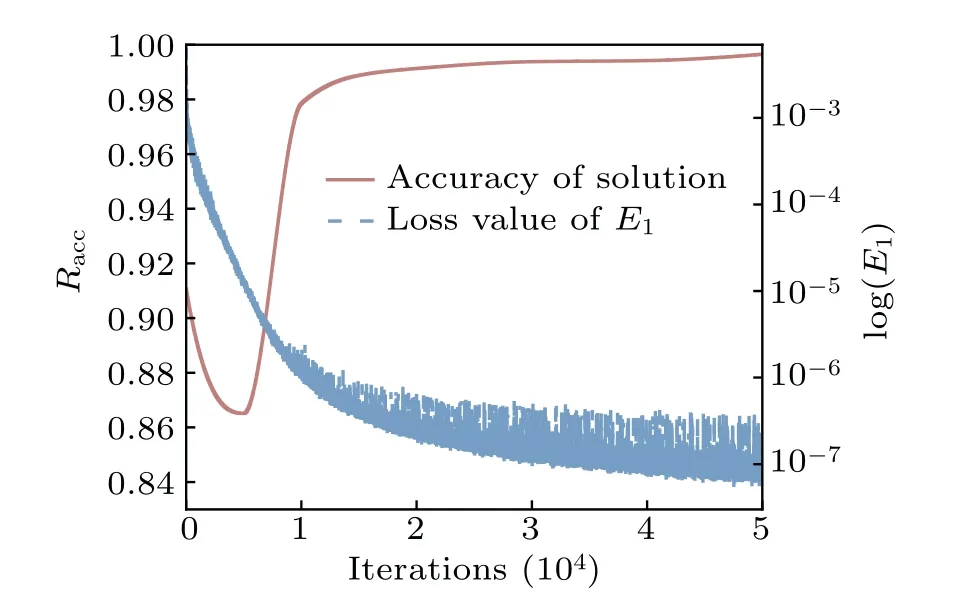
Fig.8.Evolution of solution accuracy and the value of the loss function with the number of iterations.The solid line signifies the accuracy,corresponding to the left axis, while the dotted line indicates the value of the loss function,aligned with the right axis.
As can be seen from Fig.8, the accuracy of the solution exceeded 99.13%after 2.0×10⁴iterations and the calculation time was less than 1560 s(including pre-training),which implies that the method is still applicable in high-dimensional situations.The final result has an accuracy of approximately 99.65%, which is remarkable for high-dimensional systems.The accuracy of the solution decreased in the early training stage due to the fact thatE1of the pre-trained model is so large that, the effect ofE2in fitting the NN was temporarily overwhelmed.When the value ofE1returned to a normal level,the supervision points begin to play a role in suppressing the generation of zero solution,and the accuracy of the solutions start to improve.The accuracy of the final solution is demonstrated by showing results near the center of the 6D state space.It is obvious that the DL-BPK method is still applicable in highdimensions,and the accuracy is maintained at a good level.At the same time,it is worth noting that we only trained 5.0×10⁴times on the basis of the pre-trained model to achieve satisfactory accuracy, which will be very difficult for other methods.To further illustrate the applicability of this method in higherdimensions,the slice probability density far from the center of the 6D state space is shown in Fig.9.
As shown in Fig.9, in the region where the probability density approaches zero,the result acquired from the proposed DL-BPK still shows good agreement with the exact probability distribution.
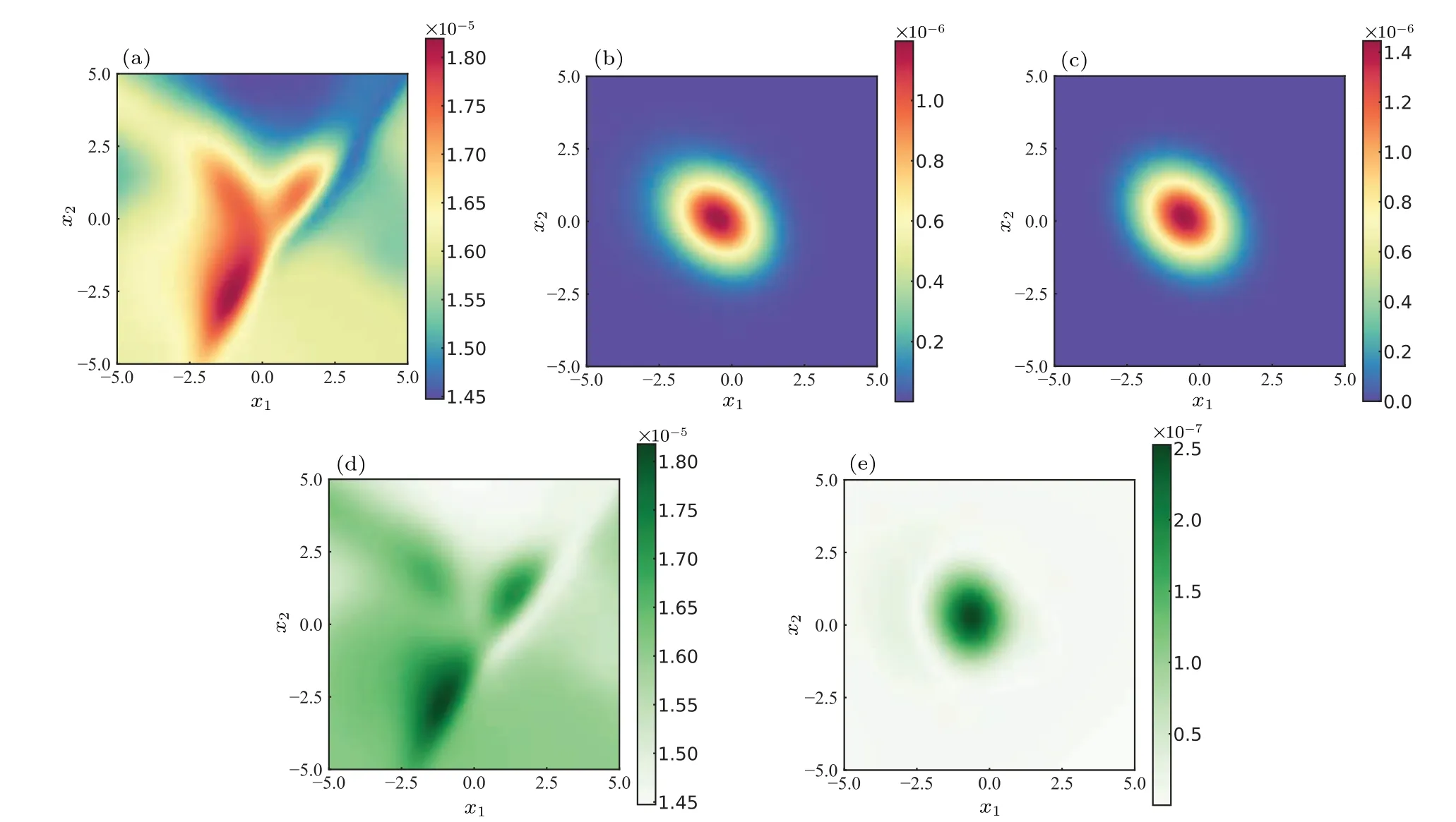
Fig.9.Comparing probability densities on slices far from the center in 6D state space: (a) p(x1,x2|y1 =y2 =x3 =y3 =2.0) of pre-trained model;(b)p(x1,x2|y1=y2=x3=y3=2.0)of DL-BPK method;(c)analytical p(x1,x2|y1=y2=x3=y3=2.0);(d)solution error of panel(a);(e)solution error of panel(b).
3.4.A 8D system
The applicability of the DL-BPK method in higherdimensions is of great interest.Nevertheless, it is generally challenging to verify the results in high-dimensional situations, so a linear system with known exact distributions is chosen.[23]Considering the following SDE with linear deterministic part
whereΓi,i=1,...,Ndenotes the independent standard Gaussian white noise with zero mean-value, whileσ=1 signifies the noise intensity.X=(x1,x2,...,xN)Tis the column vector of variables.The deterministic part of system(20)has the matrix formAX.The invariant probability measure of system(20)satisfies
We determineΣby solving the Lyapunov equationAΣ+ΣAT+2I=0.Given the symmetry ofA,we can representΣasin Eq.(21).The dimensionNwas set to 8.It is almost impractical to perform uniform sampling at such high dimensions,even if the sampling is extremely sparse.Hence,we use random sampling from within the domain and from the boundary to generateTDandTB,containing 1.0×10⁶and 5.0×10⁵points respectively.Then,Tsalso is used as the training set in this experiment, which has 1.0×10⁵data sampled from the trajectory of Eq.(20).The probability density ofTSis obtained through MCS and the penalty factor is set toλ=0.01.The final solution was achieved through 2×10⁴times of pre-training and then 5×10⁵times of training which took nearly 30 hours.The training cost in this experiment is enormous,although it is only two dimension higher than system (17).And we are more interested in the applicability of high-dimensions, so there will be a sacrifice in efficiency to some extent.
It can be seen from Fig.10 that the agreement between the exact solution and DL-BPK solution is acceptable only near the central slice,and when it is far from the central slice,the numerical value is no longer of the same magnitude as the exact solution.Such a phenomenon might result from the fact that more representative training sets for NNs are required when solving higher-dimensional systems.Assuming 100 grids are divided into each dimension, there will be 1016points in the entire space.Therefore, for an 8D system, the amount of data of points in its space is extremely terrifying.This results in the training set used in this paper being unable to quickly traverse the entire space,which leads to an increase in training costs.Therefore, how to sample more representative data is still a problem that must be solved when facing high-dimensional problems.This is also the focus and direction of our future research.
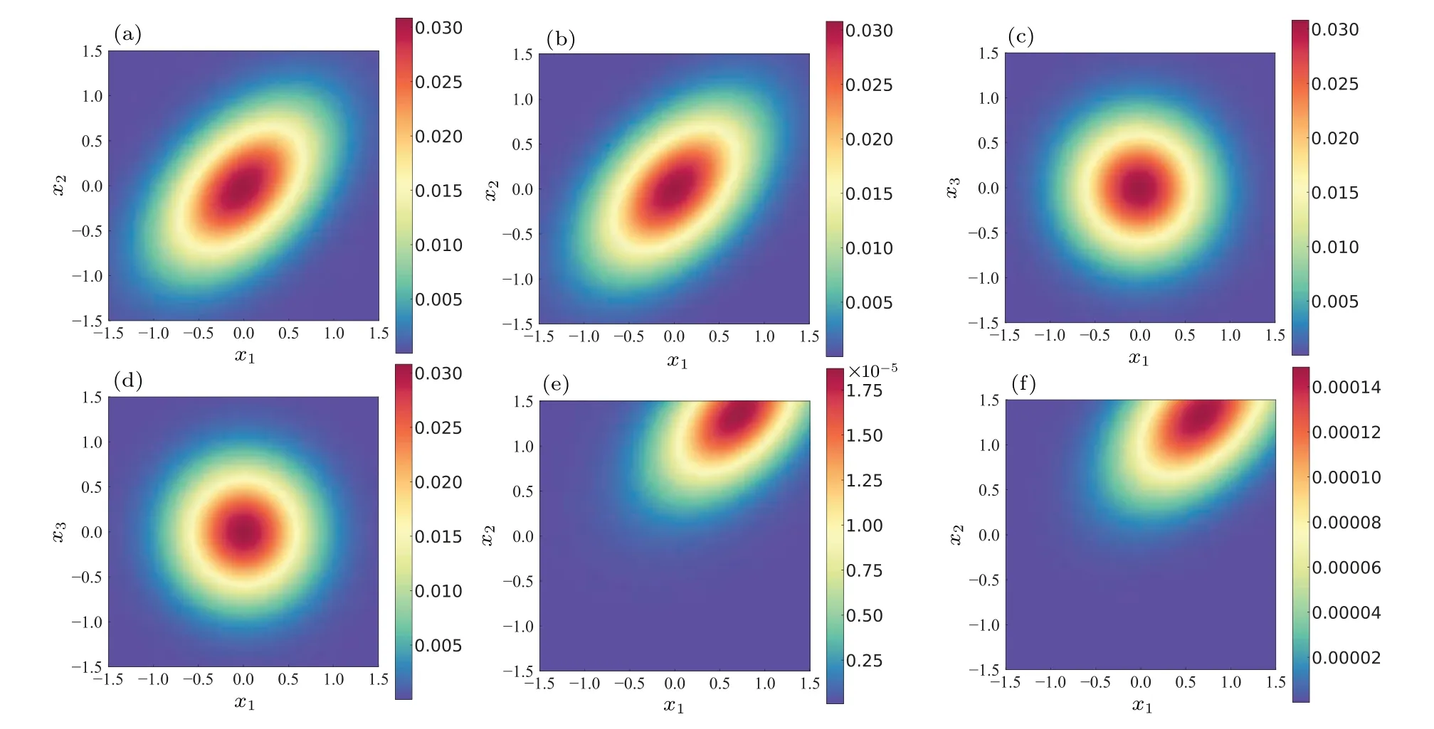
Fig.10.Results for system(20)with N=8: (a) p(x1,x2|x(3~8)=0)of DL-BPK;(b)analytical p(x1,x2|x(3~8)=0);(c) p(x1,x3|x(2,4~8)=0)of DL-BPK;(d)analytical p(x1,x3|x(2,4~8)=2.0);(e) p(x1,x2|x(3~8)=2.0)of DL-BPK;(f)analytical p(x1,x2|x(3~8)=2.0).
4.Discussion
The advantages of the proposed DL-BPK method in computational efficiency and accuracy have been demonstrated in the previous section.Further experiments are also conducted to investigate the impact of different numbers of supervision points on the robustness of the method.In this section, the following two aspects of the DL-BPK method are studied,respectively: (i)the significance of the pre-trained model to the calculation performance,and(ii)the role of the penalty factors in the proposed method.
4.1.The significance of pre-training
The influence of the pre-trained model on the accuracy and speed is discussed first.We will discuss the systems(12)and (17), which represent the low-dimensional and highdimensional cases respectively.The experimental conditions are identical to those described in Section 3, except that the pre-training step is canceled,so that the impact of pre-training on accuracy could be reflected.It should be noted that in the absence of pre-training scenarios,pθ1(XLi)is obtained by MCS.
Additionally, the total training times of NNs with and without pre-training are the same.We can clearly observe in Fig.11 that the accuracy of the results obtained without pretraining is much lower than that with pre-training.Especially for system(17),which is a 6D system,the results without pretraining are extremely poor.This test shows that the presence of pre-training is vital for the enhancement of solution accuracy as well as efficiency,which is particularly evident in highdimensional situations.
Since the existence of the pre-training step casts great influence on solution accuracy, it is necessary to study further the impact of the errors of the pre-trained model on the final result.According to Subsection 2.2, the accuracy of the pre-trained model is primarily determined by the prior knowledge obtained by the MCS.Therefore,adjusting the number of MCS steps to affect the accuracy of the pre-trained model is reasonable.For system(12), the prior knowledge is obtained by MCS with 103,104,5×104,and 105steps respectively,and these four cases are referred to as case I–IV.Then the models that have been pre-trained for 2000 and 5000 times are used as the basis for subsequent training,and the results are shown in Fig.12.It can be seen from Figs.12(b)and 12(c)that the error of the pre-trained model hardly interferes with the final calculation in terms of convergence speed and ultimate error.The accuracy of case I in Fig.12(c) fluctuates significantly in the initial stage, mainly due to highly rough prior knowledge(induced by few iteration steps of MCS)which leads toE1increasing with iteration during the pre-training process as shown in Fig.12(d).However,it is gratifying that the introduction of FPK differential operator can quickly repair the NNs in the subsequent training.
In short, the pre-trained model facilitates quick fitting of the NN by jumping out of local saddle points when solving high-dimensional systems,and the inclusion of the pre-trained model is essential for the accuracy of the final result.However, the accuracy of the pre-trained model is of less importance since it has little impact on the final result,which means that the DL-BPK method is not entirely determined by the accuracy of MCS and has excellent self-correction ability.
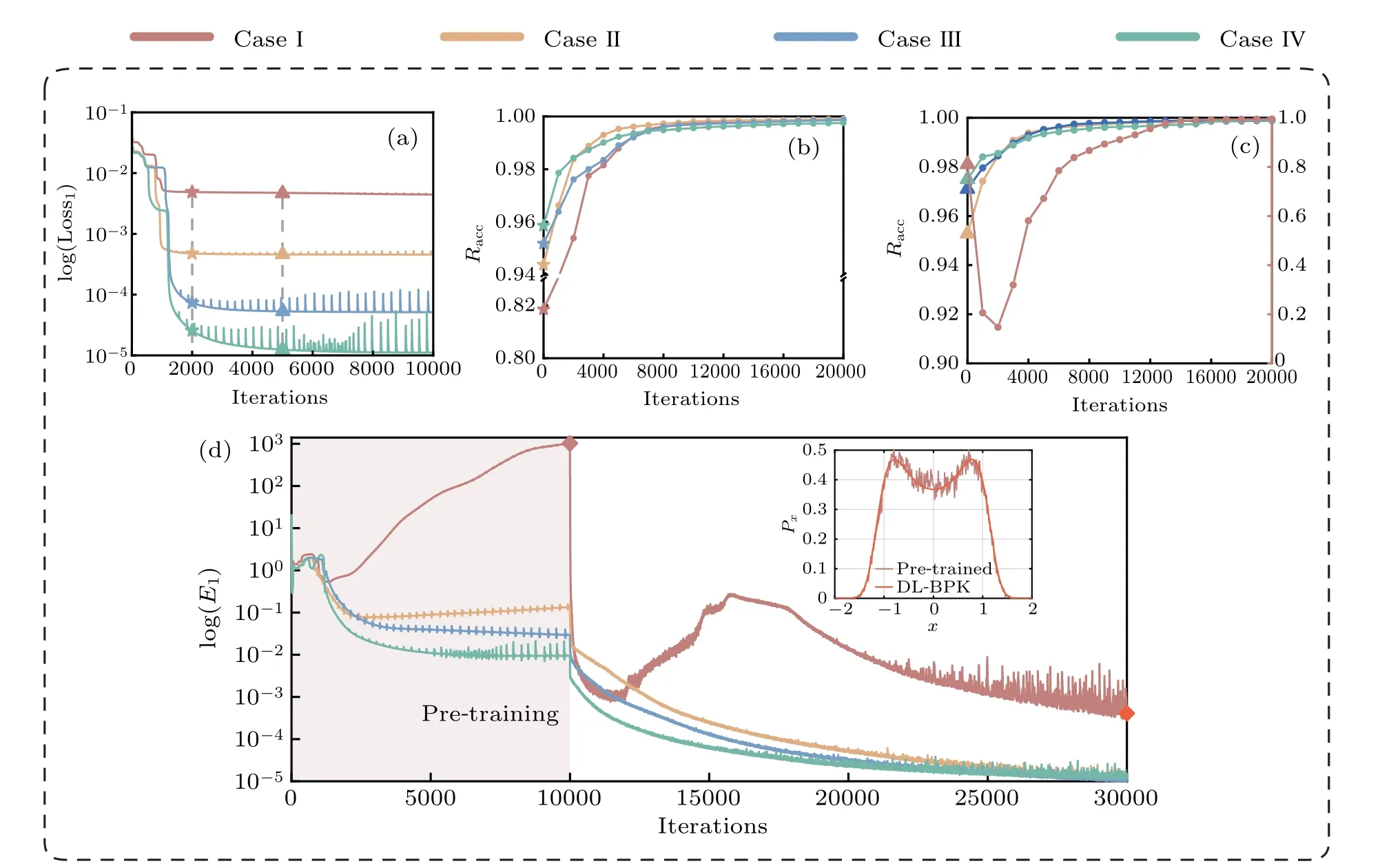
Fig.12.The effect of errors of the pre-trained PDF on the final NN PDF in terms of convergence speed and ultimate error: (a)evolution of the value of Loss1 with iterations in pre-training process;(b)–(c)after 2000 and 5000 pre-training respectively,the variation of solution accuracy with iterations in the subsequent training;(d)evolution of the value of E1 with iterations in entire training process.
4.2.The role of the penalty factors
The effect of the penalty factors is discussed using systems (12), (17), and (20).It is important to mention that we have excluded system (15) from consideration due to the absence of an exact solution and the resulting inability to quantify the accuracy of its outcomes.The FPK equation is solved with penalty factors of different magnitudes, and other relevant parameters and settings remain the same as in Section 3.Each experimental result is the average of three independent trials and the final results are shown in Fig.13.
It can be seen that penalty factors of different magnitudes have little impact on the results of each system.Only when the penalty factor is 1×10?4, is the result accuracy of a 2D system extremely poor.The reason is that the probability density value at the local maximum point of the 2D system is small.When the penalty factor is too small,it may cause the supervision points to lose its ability to prevent zero solution.However,the specific rules for setting the penalty factor need further investigation,which may relate to the error and the magnitude in the probability density at the supervision points.In general,it will not happen that an unreasonable setting of penalty factors causes the inability to solve the correct results.Compared with the DL-FP method,the method proposed does not entirely rely on penalty factors.The primary function of the penalty factor is controlling the NN to fit in the direction of the FPK differential operator, which is crucial to improve the smoothness and accuracy of the results,and to prevent zero solution.
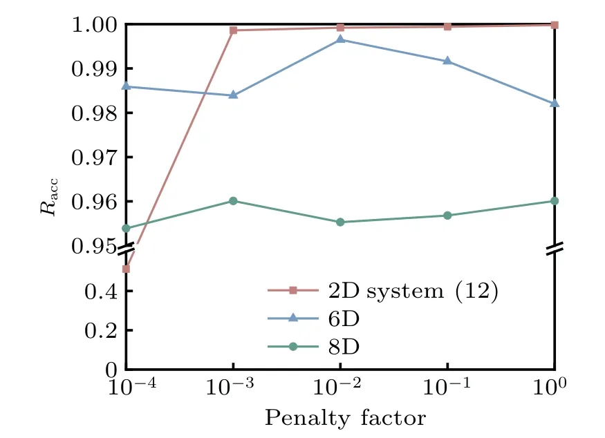
Fig.13.The impact of penalty factors on different systems.
5.Conclusions
This paper introduces a numerical method,DL-BPK,designed to solve FPK equations efficiently and accurately, and with applicability in high-dimensional systems.The basic idea is using prior knowledge to obtain a pre-trained model, and taking the discretization form of the FPK equation as a loss function to ensure the smoothness of the solution.To avoid the generation of zero solution, the supervision points with probability density are taken as a term in the loss function.The accuracy of DL-BPK solution in the first 2D system, as well as other 6D and 8D systems reaches 99.97%, 99.65%,and 95.55%,respectively.For the remaining 2D toggle switch system,DL-BPK solution also achieves good consistency with the MCS results.The proposed method outperformed other NN-based methods for solving the FPK equation in both accuracy and efficiency.
Due to the introduction of supervision points in the loss function,the influence of the number of points and the selection rules on the results are studied.The results indicate that the points with the highest probability density within a specific range,the local maximum points of PDF,should be selected as the supervision points.Next, we delved into the significance of pre-trained model.All the results validate our conjecture and confirm the practicality of the proposed method.This provides some implications for solving higher-dimensional problems.Besides, the impact of penalty factors on results and possible setting rules are also discussed.The results indicate that different levels of penalty factors will have different impacts on the results.In general, and the recommended value lies between 0.1 and 1×10?4.Proper selection of penalty factors will bring the focus of NN training closer to the FPK form, facilitating the smoothness of the solution.Moreover,the setting of penalty factors also depends on the probability density of the supervision points, which is determined by the system equation and noise intensity.Specific and strict rules still need to be studied through more models.
To compare with the exact solution,relatively simple dynamic systems are used to test the accuracy of the DL-BPK method,and future work will focus on the solution of complex nonlinear dynamic systems.It should be pointed out that since the focus of this study is not on how to sample datasets effectively, there are some data explosion issues in 8D and higher dimensional systems,which undoubtedly have a significant effect on computational cost and may limit the application of this method in higher dimensions.Therefore, data optimization and more efficient sampling methods will be the focus of our future research.Additionally, this paper only studies the FPK equation for the case of standard Gaussian white noise,and we will further consider the cases under non-Gaussian colored noise or extreme events.
Acknowledgement
Project supported by the National Natural Science Foundation of China(Grant No.12172226).
猜你喜歡
動漫界·幼教365(大班)(2024年2期)2024-05-16 08:53:32
兒童時代·快樂苗苗(2022年1期)2022-03-11 08:24:56
小天使·六年級語數(shù)英綜合(2020年8期)2020-12-16 02:59:28
美育學刊(2019年2期)2019-03-29 03:51:36
小獼猴智力畫刊(2017年5期)2017-05-25 10:21:40
專用汽車(2016年1期)2016-03-01 04:13:13
China Pictorial(2015年11期)2015-12-11 16:09:59
作文周刊·小學一年級版(2014年48期)2014-07-06 17:05:57
小青蛙報(2006年1期)2006-02-18 05:06:08

- Chinese Physics B的其它文章
- High responsivity photodetectors based on graphene/WSe2 heterostructure by photogating effect
- Progress and realization platforms of dynamic topological photonics
- Shape and diffusion instabilities of two non-spherical gas bubbles under ultrasonic conditions
- Stacking-dependent exchange bias in two-dimensional ferromagnetic/antiferromagnetic bilayers
- Controllable high Curie temperature through 5d transition metal atom doping in CrI3
- Tunable dispersion relations manipulated by strain in skyrmion-based magnonic crystals