A NON-LOCAL DIFFUSION EQUATION FOR NOISE REMOVAL*

Dong YAN (嚴(yán)冬) Boying WU (吳勃英)

1.School of Mathematics,Harbin Institute of Technology,Harbin 15000,China

2.School of Mathematics,University of California at Irvine,Irvine 92697,U.S.A.

E-mail: sjfmath@foxmail.com;mathgzc@hit.edu.cn;mathywj@hit.edu.cn;dyan6@uci.edu;mathwby@hit.edu.cn

Abstract In this paper,we propose a new non-local diffusion equation for noise removal,which is derived from the classical Perona-Malik equation (PM equation) and the regularized PM equation.Using the convolution of the image gradient and the gradient,we propose a new diffusion coefficient.Due to the use of the convolution,the diffusion coefficient is non-local.However,the solution of the new diffusion equation may be discontinuous and belong to the bounded variation space (BV space).By virtue of Young measure method,the existence of a BV solution to the new non-local diffusion equation is established.Experimental results illustrate that the new method has some non-local performance and performs better than the original PM and other methods.

Key words image denoising;non-local diffusion;BV solutions;Perona-Malik method

1 Introduction

Images are inevitably affected by noise in the process of acquisition and transmission,so that image denoising is an important task in image processing.The main difficulty in image denoising is to preserve the details of information such as the edges and textures of the original image from the noisy observation.Most of the time,those details of information are of vital importance in subsequent image processing tasks,such as image segmentation and image restoration.

Research on image denoising based on partial differential equations (PDE) has developed extensively over the course of the last thirty years.Osher,in [1],proposed a pioneering denoising model by a total variation (TV) method.Later,Vese,in [2],summarized a family of denoising methods based on a variational PDE,then more in-depth studies on its theoretical background were proposed in [3] and [4],and the relevant numerical methods were proposed in [5–8].After that,denoising methods based on second-order equations were generalized to other types of PDEs,such as fourth-order PDEs [9–11] and fractional PDEs [12–14].

Perona and Malik proposed an anisotropic diffusion equation [15] (the PM method) as follows:

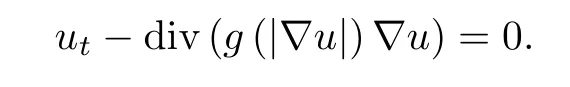
Hereg(s) is a diffusivity function with the form

The anisotropic diffusion enables the PM equation to detect the edge area of a noisy image and implement an edge preserved diffusion.Moreover,the diffusion approach of the PM equation was proved to be forward-backward,i.e.,the edge area can not only be preserved,but also be enhanced.However,this edge enhancement also leads to artificial phenomena;new features are added to the restored images so that it no longer preserves the original information.As a result,there will appear the “staircase” and “speckle” effects in the restored images.A regularized PM equation (RPM [16]) was proposed to avoid forward-backward diffusion in the original PM equation by refining the diffusivity function fromg(|?u|) tog(|?Gσ*u|),whereGσis a Gaussian function

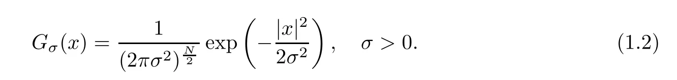
With Gaussian convolution,the diffusivity becomes totally forward.Furthermore,the RPM method becomes a well-posed problem,and the solution of the RPM equation is smooth,which effectively avoids the “staircase” effect of the PM method.Unfortunately,this smooth solution sometimes will result in blurry edges in the restored images.

Guidotti,in [17–19],regularized the diffusivityg(|?u|) in the PM equation by fractional derivativesg,and proved in a one dimensional situation that the new equation could be changed from a PM equation to a linear heat equation,as∈goes from 0 to 1.Later,Guidotti,in [20],proposed the “milder” regularized PM method by modifying the diffusivity function of the PM equation into

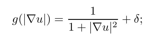
the “milder” regularization preserves the forward and backward diffusion property of the PM method but enables the equation to remove the “staircase” and “speckle” effects.Furthermore,in [21],the authors extended this“milder” regularization diffusivity to

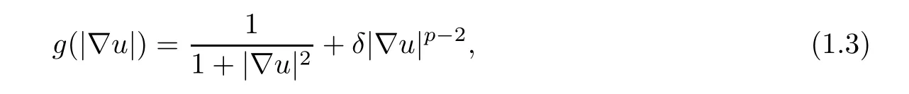
wherep∈[1,+∞).

In this paper,we consider a new model for noise removal:

Define ΩT:=Ω×(0,T),where Ω ?RNis a bounded Lipschitz domain with boundary?Ω,and Γ :=?Ω × (0,T).u0(x) is the initial noisy image.The diffusivity function contains both the gradient term and the convolutional gradient term,which combines the advantages of PM and RPM simultaneously.It is worth noticing that our new model is not just a trivial combination of two existing models;the properties of the solution of our model are totally different from that of the others and we will discuss this in depth in the ensuing sections.Because of the non-local term |?Gσ*u|,the new diffusion at every point depends on a neighborhood of this point.

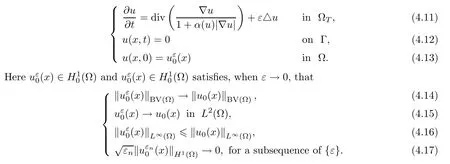
In terms of mathematical theory,we investigate the first initial-boundary value problem of diffusion equations in more general form as follows:

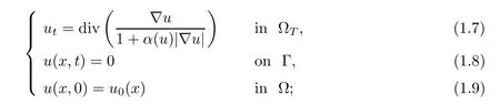
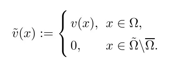
this will be denoted by P.Hereu0(x) ∈BV(Ω) with a zero trace on?Ω.We also have that,fi∈S(RN),and by |·| we denote the Euclidean norm and we define S(RN) to be the Schwartz space.Givenu∈L2(Ω),we extend this by zero to the whole of RNand denoteas the extended function.a(·) ∈C2[0,∞) anda(x) ≥0.Letf*～ube the convolution offand～uin RN.In particular,for the caseα(u)=|?Gσ*u|,(1.7)–(1.9)become (1.4)–(1.6).The loss of growth,however,brings some technical difficulties whenα(u)arrives at zero.We prove the existence of the solution to P for the case in whichα(u) ≥c ＞0,in theory.This means thatα(u)=|?Gσ*u|+εis allowed,for a smallε ＞0.The uniqueness is proved in a narrower class of functions than the existence.

The rest of this paper is organized as follows: in Section 2,we propose the non-local PM method.Section 3,Section 4 and Section 5 are the mathematical theory parts of the paper.We first state the mathematical preliminaries in Section 3.The existence of solutions to problem P is proved in Section 4.In Section 5,we investigate the uniqueness of solutions to problem P.Finally,Section 6 verifies the effectiveness and superiority of our proposed method by comparative numerical experiments.

2 Non-local PM Denoising Method

In this section,comparing our new model with the PM and RPM models,we discuss how our new model works and the non-triviality of our modification.

As we know,PM diffusion is forward-backward,and this creates is an ill-posed problem.An image restored by the PM method may have black and white speckles and false edges because of the backward diffusion.RPM diffusion is regularized and well-posed,and produces smoothing solutions,but this regularization property may destroy the edges in the restored image.Combining the advantages of PM and RPM,and the corresponding diffusivities,

we propose the diffusivity function

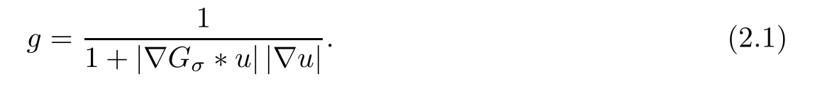
PM diffusivity only involves point-wise operation,and thus the PM equation is a local method.RPM is non-local because of the convolution.Our new model combines the two features so that it is also non-local.We name our new model the “non-local PM” (NLPM)method.

The non-triviality of our model is mainly reflected in the properties of the solutions.The solution of the PM equation may not exist,or exist but not be unique [22].The solution space of the RPM equation is theC∞space [16].However,some researchers regard the BV space as the right space for image processing [1,31].With our new diffusivity (2.1),the NLPM model is proved,in the next section,to have a BV solution,and so is similar to the TV model [1].

Next,a prototypical example is used to illustrate the edge-preserving ability of our NLPM method.Formally,one can regard the edge of an image as a function with a large gradient norm,observing that the diffusivity of the NLPM method consists of |?u|-1,so the NLPM method should undertake no diffusion on the edge area of an image,i.e.,the edge will be preserved by the NLPM method.Although this is not a strict mathematical analysis,numerical experiments enable to validate this conclusion.Now we consider that

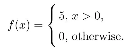
This function has a jump discontinuity atx=0,which can be regarded as an edge of the one-dimensional signalf.Also,we consider the mollified signalsfσby the Gaussian kernels(1.2) with a different parameterσ,as shown by the red lines in Figure 1.Then we use the NLPM method to process these signals;the output signals are shown as the black circled lines.One can observe clearly that the NLPM method preserves the edge very well.

Figure 1 The NLPM method enables one to maintain the jump discontinuity

Figure 2 Synthetic one-dimensional signal

Figure 3 The PM method has a “staircase” effect

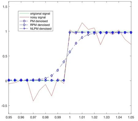
Figure 4 The RPM method mollifies the edge

Another prototypical experiment on one-dimensional signal processing demonstrates,intuitively,the differences between the PM method,the RPM method and the NLPM method.Consider the one-dimensional forms of the three respective methods as follows:

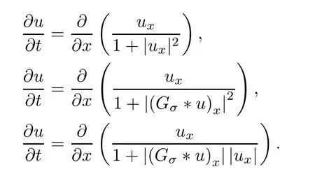
We use these equations to process a synthetic one-dimensional signal,as shown in Figure 2.Notice that this example consists of various cases such as jump discontinuities and the smooth periodic signal.Figure 3 shows that the PM method has a severe “staircase” effect in smooth intensity transition areas (i.e.,the trigonometric function part of the synthetic signal),while the RPM and NLPM methods maintain the smoothness well.Furthermore,we zoom on the discontinuous region of the signal (i.e.,the staircase function part) and put the processing results together in Figure 4.One can easily see that the RPM method mollifies the edge while the other two methods preserve the edge well.Noticing that the x-ticks in Figure 4 are close to the jump discontinuityx=1,it is natural that this phenomenon is not quite as obvious in the original figures as in Figure 3.

In addition,the parameterσin the NLPM diffusivity function (2.1) also increases the flexibility of the model.The parameterσis related to the window size of the Gaussian convolution,which shows the non-locality of the model.Whenσapproaches zero,the non-locality of the model is minimized and the equation degenerates to the original PM equation.Whenσapproaches ∞,the model is approximate to the Laplacian equation.

3 Mathematical Preliminaries

3.1 Pairings between Measures and Bounded Functions

Denote M(X) as the set of finite Radon measures on a Borel setX,and denoteM1+(X)as its subset of probability measures.As usual,LNand HN-1represent theN-dimensional Lebesgue measure and (N-1)-dimensional Hausdorffmeasure in RN,respectively.We denote M+(X) as the positive Radon measures.For allλ1,λ2∈M(X),

DenoteC0(RN) as the closure of continuous functions on RNwith compact support.The dual ofC0(RN) can be identified with the Radon measure space M(RN) via the pairing

Let the setD?Rnbe a measurable set with finite measure.A mapν:D→M(RN) is said to be weakly*measurable if the functionsfdνxare measurable for allf∈C0(RN),whereνx=ν(x).

Throughout the rest of this paper,Irepresents the identity operator in RN.

A functionu∈L1(Ω) is called a function of bounded variation if its distributional derivativeDuis a RN-valued Radon measure with finite total variation in Ω.The vector space of functions of bounded variation in Ω is denoted by BV(Ω).The space BV(Ω) is a non-reflexive Banach space under the norm ‖u‖BV:=‖u‖L1+|Du|(Ω),where |Du| is the total variation measure ofDu.

Foru∈BV(Ω),the gradientDuis a Radon measure that can be decomposed into its absolutely continuous and singular parts

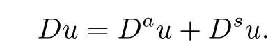
Then,Dau=?uLN,where ?uis the Radon-Nikod′ym derivative of the measureDuwith respect to the Lebesgue measure LN.There is also the polar decompositionwhereis the Radon-Nikod′ym derivative ofDsuwith respect to its total variation measure |Dsu|.

Lemma 3.1Assume thatu∈BV(Ω).There exists a sequence of functionsui∈W1,1(Ω)∩C∞(Ω) such that

(i)ui→uinL1(Ω);

(ii) |Dui|(Ω) →|Du|(Ω);

(iii)ui|?Ω=u|?Ωfor alli.

Moreover,

(iv) ifu∈BV(Ω) ∩Lq(Ω),q ＜∞,we can find functionsuisuch thatui∈Lq(Ω) andui→uinLq(Ω);

(v) ifu∈BV(Ω) ∩L∞(Ω),we can finduisuch that ‖ui‖∞≤‖u‖∞andui→uweakly*inL∞(Ω).

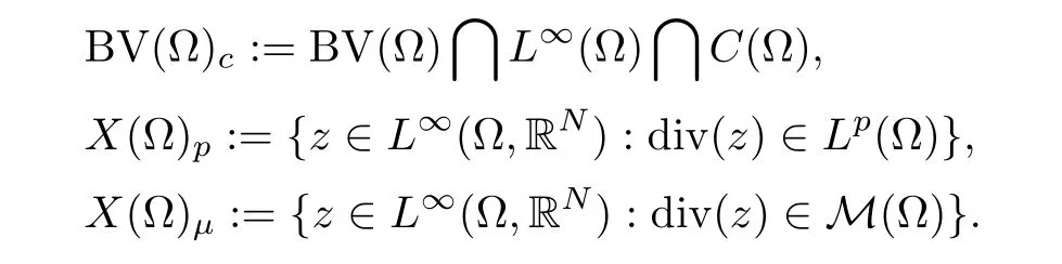
It is well known that the summability conditions on the divergence of a vector fieldzin Ω yield trace properties for the normal component ofzon?Ω.As in [23],we define a function[z,→n] ∈L∞(?Ω),which is associated to any vector fieldz∈L∞(Ω,RN) such that div(z) is a bounded measure in Ω.

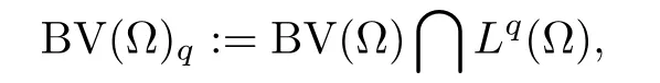
Assume that Ω is an open bounded set in RNwith?Ω Lipschitz,N≥2,and 1 ≤p≤N,Since?Ω is Lipschitz,the outer unit normal→nexists in HNa.e.on?Ω.We shall consider the following spaces:

Lemma 3.2Assume that Ω ?RNis a open bounded set with Lipschitz boundary?Ω.Then there exists a bilinear map 〈z,u〉?Ω:X(Ω)μ× BV(Ω)c→R such that

Lemma 3.3Let Ω be as in Lemma 3.2.Then there exists a linear operatorγ:X(Ω)μ→L∞(?Ω) such that

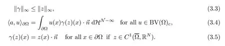
The functionγ(z) is a weakly defined trace on?Ω of the normal component ofz.We denoteγ(z) by [].

In the sequel,we shall consider pairs (z,u) such that one of the following conditions holds:

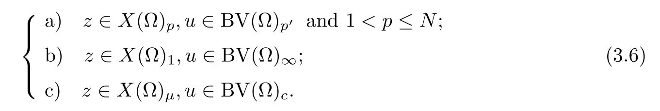
Definition 3.4Letzandube two functions such that one of the conditions of (3.6)holds.Then we define a functional (z,Du): D(Ω) →R as

Lemma 3.5For all open setsV?Ω and for all functionsφ∈D(V),one has that

and thus,(z,Du) is a Radon measure in Ω.

We give the Green’s formula relating the functionand the measure (z,Du).

Lemma 3.6Let Ω be as in Lemma (3.2).Ifzanduare two functions such that one of the conditions of (3.6) holds,then we have that

More details about the pairings 〈z,u〉?Ωand (z,Du) can be found in [23].

3.2 The Generalized Young Measure

This subsection gives a brief overview of the basic theory of generalized Young measures and recalls results that will be used later.We refer to [24] for further information about the generalized Young measures.

First,we need a suitable class of integrands.Let E(Ω;RN) be the set of allf∈C(Ω × RN)such that

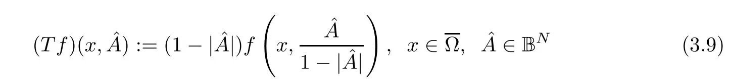
extends into a continuous function,where BNstands for the unit sphere in RN.In particular,this implies thatfhas linear growth at infinity,i.e.,there exists a constantM ＞0 (in fact,such that

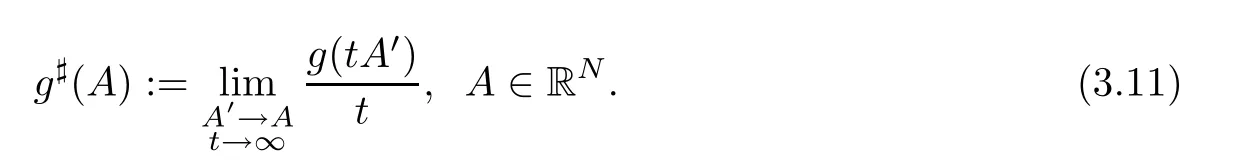
For allf∈E(Ω;RN),the recession function

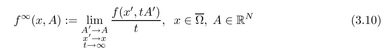
exists as a continuous function.Sometimes this notion of a recession function is too strong,so for any functiong∈C(RN) with linear growth at infinity,we define the generalized recession function as

Definition 3.7A generalized Young measure with target space RNis a tripleλ=(νx,λν,νx∞) comprising

(i) a parametrized family of probability measures

(ii) a positive finite measure

(iii) a parametrized family of probability measures(?BNdenotes the unit sphere in RN);

(iv) a mapxνxis weakly*measurable with respect to LN,i.e.,the functionx〈νx,f(x,·)〉 is LN-measurable for all bounded Borel functionsf: Ω × RN→R;

(v) a mapxν∞xis weakly*measurable with respect toλν;

(vi)x〈νx,| ·|〉 ∈L1(Ω).

ByY(Ω;RN),we denote the set of all such generalized Young measures.The parametrized measure (νx) is called the oscillation measure,the measureλνis the concentration measure,and (νx∞) is the concentration-angle measure.

The duality pairing 〈〈λ,f〉〉 forλ∈Y(Ω;RN) andf∈(Ω;RN) is defined by

The spaceY(Ω;RN) of Young measures can be considered as a part of the dual space E(Ω;RN)*(the inclusion is strict since,for instance,dxlies in E(Ω;RN)*Y(Ω;RN) whenevers≠1).This embedding gives rise to a weak* topology onY(Ω;RN)and so we say that (λj) ?Y(Ω;RN) (where) weakly*converges toλ∈Y(Ω;RN),in symbols,,if 〈〈λj,f〉〉 →〈〈λ,f〉〉 for allf∈E(Ω;RN).The setY(Ω;RN) is topologically weakly*-closed in E(Ω;RN)*.

The main compactness result in the spaceY(Ω;RN) is listed as follows:

Lemma 3.8Let (λi) ?Y(Ω;RN) be a sequence such that

(i) the functionsx〈(νj)x,|·|〉 are uniformly bounded inL1(Ω);

(ii) the sequence (λνj()) is uniformly bounded.

Then,(λj) is weakly*sequentially relatively compact inY(Ω;RN),i.e.,there existλ∈Y(Ω;RN)and a subsequence of (λj) (not relabeled) such that

Next,we define the setGY(Ω;RN) of generalized gradient Young measures as the collection of the generalized Young measuresλ∈Y(Ω;RN) with the property that there exists a normbounded sequence (uj) ?BV(Ω) such that the sequence (Duj) generatesλ,which,in symbols,we will write asmeaning that

for allf∈E(Ω;RN).

Lemma 3.9Letλ∈Y(Ω;RN) be a generalized Young measure withλν(?Ω)=0.Thenλ∈GY(Ω;RN),if and only if there existsu∈BV(Ω) with

and for all quasiconvexg∈C(RN) with linear growth at infinity,the following Jensen-type inequalities hold:

(i)

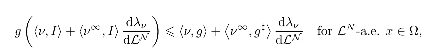
(ii)

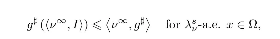
whereis the singular part ofλwith respect to the Lebesgue measure LN.

We remark that for both flavors of recession function,one can drop the additional sequenceA′→Aif the functional is Lipschitz continuous (see [25]).

Givenu∈BV(Ω),denote thatσDu:=(δ?u,|Dsu|,δp) ∈GY(Ω;RN) and.δAis denoted as the Dirac measure on RNgiving unit mass to the pointA∈RN.

Throughout the rest of this paper,uΩrepresents the trace ofu∈BV(Ω) on?Ω.

Referring to [26],Corollary 4,we have the following necessary lemma:

Lemma 3.10AssumeX?B?Ywith compact imbeddingX?B(X,BandYare Banach spaces).

i) LetFbe bounded inLp(0,T;X),where 1 ≤p ＜∞,and letbounded inL1(0,T;Y).ThenFis relatively compact inLp(0,T;B);

ii) LetFbe bounded inL∞(0,T;X),where 1 ≤p ＜∞,and letbounded inLr(0,T;Y) wherer ＞1.ThenFis relatively compact inC(0,T;B).

4 Existence

This section is divided into four subsections.In Subsection 4.1,we list the main results.In Subsection 4.2,we employ the regularization method and prove the existence of weak solutions of the auxiliary problems.In order to obtain the solution of problem P,some regular estimates for weak solutions of the auxiliary problems are also necessary in Subsection 4.3.Finally,we prove the main two theorems (Theorem 4.4 and Theorem 4.5) in Subsection 4.4.

4.1 Main Results

For the sake of simplicity,throughout the rest of this paper we use the notation

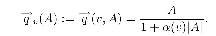
wherev∈L2(ΩT),A∈RN.

Definition 4.1A measurable functionu: (0,T) × Ω →R is a strong solution of (P) in ΩTifu∈C([0,t],L2(Ω)),u(0)=u0,u′(t) ∈L2(Ω),u(t) ∈BV(Ω) ∩L2(Ω) a.e.t∈[0,T],and there existsz(t) ∈X(Ω)1with ‖α(u)z‖∞≤1,satisfying,for almost allt∈[0,T],that

Definition 4.2A generalized Young measure valued solution of P is a pair (u,λ),whereu∈L∞(0,T;BV(Ω) ∩L2(Ω)),,and,for almost allt∈(0,T),λ=(ν,λν,ν∞)x,tis a parametrized family of generalized Young measures inY(Ω;RN) such that

Remark 4.3If (u,λ) is a generalized Young measure solution,and,for almost allt∈(0,T),λ∈GY(Ω;RN),we say that (u,λ) is a generalized gradient Young measure solution.

Theorem 4.4Givenu0∈BV(Ω) ∩L∞(Ω) with a trace of zero on?Ω,then there exists a generalized Young measure solution of P for everyT ＞0.

Theorem 4.5Suppose that all the assumptions of Theorem 4.4 hold.This admits a strong solution of P for everyT ＞0.

4.2 Weak Solution for Auxiliary Problem

We use Pεto denote the following auxiliary problem:

First,we are going to prove that there exists a weak solution (in that usual sense) of Pε.For anyv∈L2(QT),we denoteu=T vas the solution to the following problem:

By the usual theory of monotone operators,there exists a uniqueu=T v,andu∈L2(0,T;∈L2(0,T;H-1(Ω)).The following estimate holds:

According to the definition of weak solutions,

Takingφ=u,we have that

whereMis a constant independent ofεandT.It follows that

whereCis a constant independent ofεandT,we arrive at

Applying the compact embedding theorem of Aubin-Lions (see also Lemma 3.10),we get thatW(0,T) is precompact inL2(ΩT).Let us now consider the mappingT:L2(ΩT) →L2(ΩT).Based on Schauder’s fixed point theorem,it is clear that this mapping will have a fixed point provided that it is continuous.To prove this,note thatu1=T(v1),u2=T(v2).According to(4.18),taking the texting functionφ=u1-u2,it follows that

Hence,by (4.25),(4.26) and Young’s inequality,we have that

which proves the continuity of the mappingT,and thus that there exists a weak solutionuεto the problem Pε.On the other hand,using Gronwall’s inequality,(4.27) ensures the uniqueness of Pε.

4.3 Regularity for Weak Solution of Pε

In order to obtain the general Young measure solution of P,some estimates are also necessary.

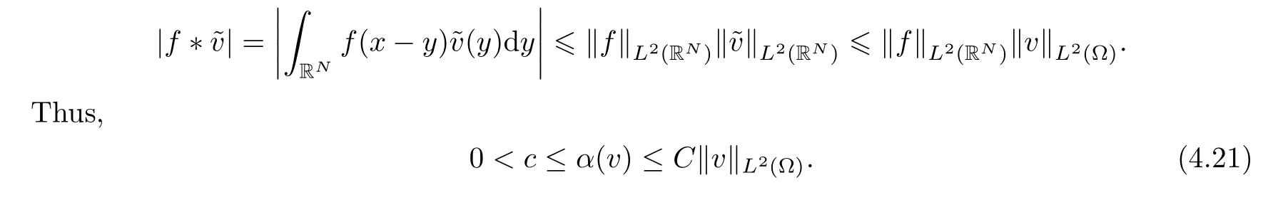
SinceL2(0,T;H-1(Ω)) is the dual space ofL2,for everyw∈L2(0,T;H-1(Ω)),it follows that

ProofBy the definition of the weak derivative off*and Fubini’s Theorem,for everyφ∈D(ΩT),one has that

On the other hand,

Collecting all of these facts,we obtain (4.28).

and this implies (4.29). □

Lemma 4.7Ifuεis a solution of Pε,then

whereCis a constant independent ofε.

ProofLet us use the notation

Multiply relations (4.18) byut.This gives the equality

We use the formulas

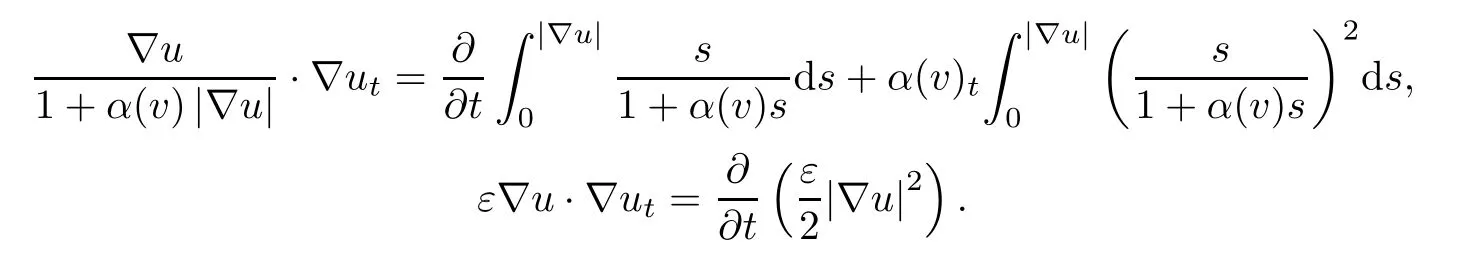
Substituting these into (4.32),we rewrite it in the form

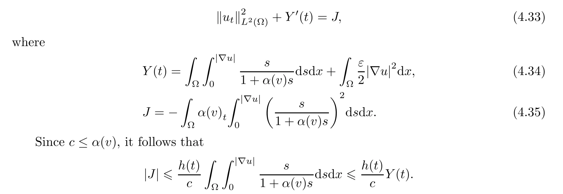
On the other hand,by Lemma 4.6,

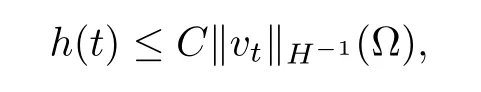
Thus,the functionY(t) satisfies the differential inequality

Omitting the nonnegative terms on the left-hand side,we estimateY(t) by using Gronwall’s lemma.The estimate follows from the integration of (4.36) over the interval (0,T). □

4.4 Letting ε →0

Proof of Theorem 4.4We set

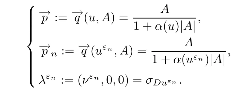
According to Lemma 3.8 and Lemma 4.7,for almost allt∈(0,T),we can extract from{uεn} and {νεn} a subsequence (still labeled {uεn} and {νεn}) such that

whereλ=(ν,λν,ν∞).

which converges to zero uniformly in.Together with (4.42),it follows that

Therefore,by (4.39) and (4.41),we get that

we obtain that

Therefore,

Step 2 Sinceut=div〈ν,〉,in D′(Ω),withut∈L2(Ω),we get that

Observe that,by (4.45) and Lemma 4.7,we obtain that

By (4.47),we have that

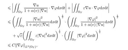
Combining (4.37),(4.41) and (4.46),we get that

On the other hand,by Green’s formula of Lemma 3.6,it follows that

Hence,by (4.52),(4.53),(4.54) and (4.55),lettingn→∞,we have that

Furthermore,by the arbitrariness ofφand the definition of～u,

Proof of Theorem 4.5To prove Theorem 4.5,we only need to prove that the generalized gradient Young measure solution in Theorem 4.4 is also a strong solution to problem P.As in the proof of Theorem 4.4,one has that

Hence,by Green’s formula of Lemma 3.6,we obtain that

With this,and

we have that

Therefore,

so its absolutely continuous part is

By choosingA=?u(x) ±∈ξ,?ξ∈RNand letting∈→0+,we obtain that

which implies (4.2).

According to (4.49) and (4.56),we have that

Then,it follows that

With this,and by

we have that

On the other hand,by (4.66),we have that

with |Ds| -a.e.in.Thus,

This implies that

Sinceu∈BV(Ω),by the boundary trace theorem (see Theorem 3.87 in [27]),we get that

Lettingz=〈ν,〉,and combining (4.61),(4.62),(4.67) and (4.68),we complete the proof.□

5 Uniqueness Results

The uniqueness is proved in a narrower class of functions than the existence.However,since the proof of Theorem 5.1 is practically independent of the proof of existence,the regularity onutis less restrictive.

Theorem 5.1There is at most one solution (in the sense of Definition 4.1 or Definition 4.2) to the problem P in the class

Proof Actually,a solution in the classW(ΩT) is also a weak solution in usual sense.Let bothu1andu2be weak solutions of P.Then one has that

where 〈·,·〉 denotes the dual product ofH-1(Ω) and

By some calculations,we get that

Collecting all of these facts,byα≥c ＞0,we obtain that

Thus,by (4.26),we have that

whereCis a constant and

Observing thatλ(t) ∈L1(0,T),by Gronwall’s inequality,it follows that

6 Numerical Scheme and Experiments

In this section,the PM scheme in [15] and a fast numerical scheme are used to implement our NLPM method.Furthermore,we compare our NLPM method with other denoising methods through experiments on different types of images.It is worth noting that,starting from this section,we introduce a positive modifier parameterKinto our NLPM diffusivity function (2.1),as the original PM diffusivity (1.1) did.More specifically,the modified diffusivity

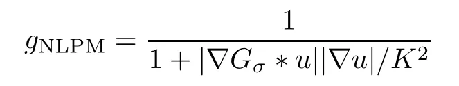
will be used in our experiments.The reason we add the modifierKis to enhance the flexibility of our NLPM method.In order to maintain the fairness of the comparison experiments,we add the modifierKto all the other methods,and adjust the parameters in order for each to reach its best results.The analytical results we proved in the previous sections can be viewed as a special case of whenK=1.We will carefully discuss the selection of parameters in Section 6.3.

6.1 Numerical Schemes

(1) PM scheme (PMS)

Similarly to the numerical scheme in [15],which was originally introduced to implement the PM method,and thus called the “PM scheme”,the scheme that follows is used for our NLPM method.

First,the gradient terms ofuandGσ*uare respectively discretized into four orthogonal directions: north,south,east and west.Assume that the width and length of the images areIandJ,respectively,and also assume that the spatial step sizes arehx=hy=1.

For 0 ≤i≤I,0 ≤j≤J,

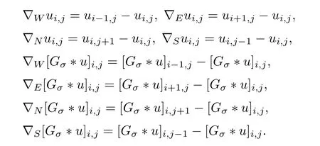
Then,we denote Λ ∈Ω={N,S,E,W} as any of the four directions,and defineas

Finally,the NLPM equation is put into a simple form as follows:

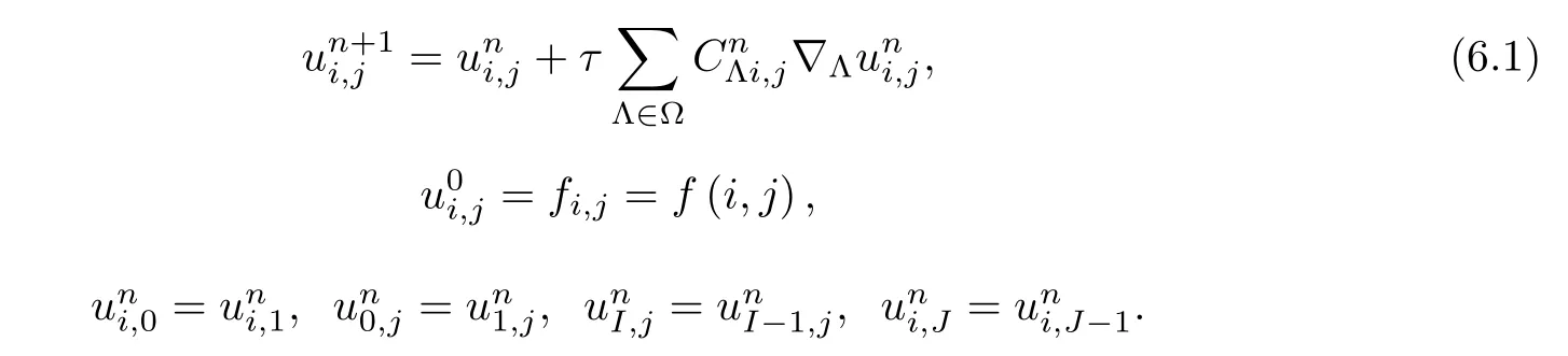
Hereτis unit time step,and 0 ≤τ≤is required to ensure that the scheme is stable.

Furthermore,if we denoteUn∈RIJas the vector with entries,then we can rewrite equation (6.1) as the matrix form

whereIis aIJ×IJidentity matrix,andA(Un) with respect toUnis a negative semidefiniteIJ×IJmatrix derived from the diffusion process at time leveln.

The PMS is a very simple and intuitive scheme to implement our new model,however since PMS is an explicit scheme with a fixed time step size,it suffers from a strict time step restriction which will cause a severe inefficiency.Therefore,we use another numerical scheme which can realize a rapid implementation for our NLPM method.

(2) Fast explicit diffusion scheme (FED)

According to Grewenig et al.[28],splitting a long fixed time step iteration into several variant time step cycles (i.e.,the FED cycles) will speed up the implementation,as well as maintain the stability.More specifically,the corresponding FED scheme for our NLPM model is as follows (given that the default spatial step sizehin image processing is 1):

1) Input: total processing timeT,the number of FED cyclesM,noisy imagef.

2) Initialization: letU0be the vector generalized byf.

3) Iteration: fork=0,···,M-1,

a) Find the current diffusion matrixP,whereP=A(Uk),according to equation (6.2).

b) Find the largest moduleμmof eigenvalues ofP(i.e.,μm=maxi|μi|,whereμiis the eigenvalue ofP).

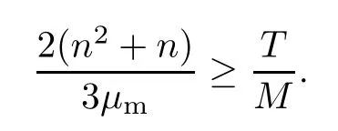
c) Find the smallestnsatisfying that

d) Compute

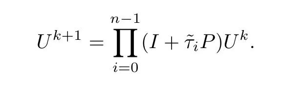
f) Do one FED cycle:

End

6.2 Numerical Experiments

We use peak signal-to-noise ratio (PSNR) to measure the effectiveness of different image denoising methods:

Hereuois the noise-free image,?uis the denoised image,andMandNare the width and length of the images,respectively.

First we compare the results of our NLPM method implemented by two schemes introduced in Section 6.1.We use these two methods (i.e.,NLPM implemented by the PMS scheme,and NLPM implemented by the FED scheme) to process the images shown in Figure 5.For each method,the iteration is stopped when the maximal PSNR value is attained.The PSNR results,processing time and corresponding parameters are listed in Table 1.We can find that the FED scheme sharply reduces the processing time of the PMS scheme,however,the PSNR of the FED scheme drops by around 0.2 -0.5 dB;this is a compromise of fast implementation.

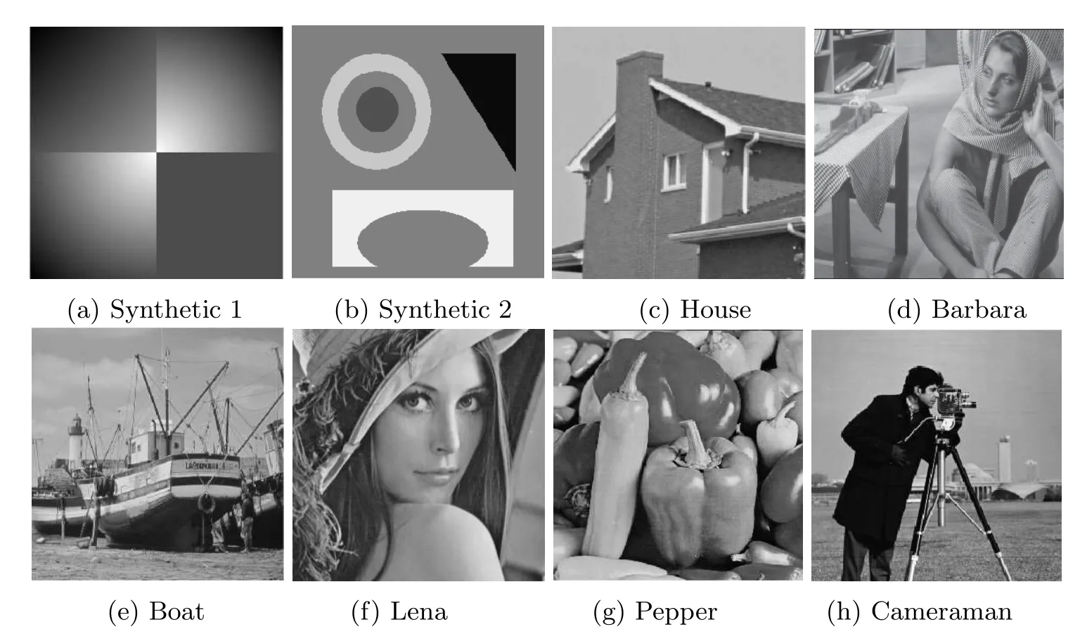
Figure 5 Test images used in comparison experiments of the PMS and FED schemes

Tabld 1 Test results between the PMS and FED schemes.All of the test images are from Figure 5.τPMS is the time step size of the PMS scheme,IterPMS is the total iterations of the PMS scheme,TFED is the total processing time of the FED scheme,MFED is the number of FED cycles,σNLPM is the parameters of the Gaussian in our NLPM method

Furthermore,to verify the effectiveness of our NLPM method,we perform comparison experiments among several different image denoising methods.In the experiments,we care more about PSNR comparison for the different methods rather than the processing time.In order to make a fair comparison between different methods,we uniformly use the simple explicit finite difference schemes for implementation (i.e.,PMS for NLPM).The corresponding parameters are set to reach the maximal PSNR for each method.

We first add Gaussian noise with a standard deviation 25 to a clean synthetic image,as shown in Figure 6(a).Then Figures 6(b)–6(d) show the denoising results of PM,RPM and our NLPM method,respectively.To make a detailed comparison,we zoom on the restored images to compare the detail performance of our NLPM method with the other two diffusion methods.Figures 7(a) and 7(e) are restored images of the PM and NLPM methods,respectively.We box three pairs of local blocks in these,and display in pairs the rest of the subfigures of Figure 7.Figures 7(b) and 7(c) demonstrate that there exists a “staircase” effect in PM restored images,while this kind of oscillation is well avoided by the NLPM method,as shown in Figures7(f)and 7(e).Figures 7(d) and 7(h) demonstrate that NLPM method can avoid black and white“speckle” effect occurring in PM restored images.Figure 8 compares the performance of the RPM and NLPM methods.From Figures 8(b) and 8(c) we can see that,in the edge areas,the RPM method has serious blurring;the contrast of two adjacent colors becomes much less obvious.Figures 8(e) and 8(f) demonstrate that the NLPM method can preserve the edge area much better.

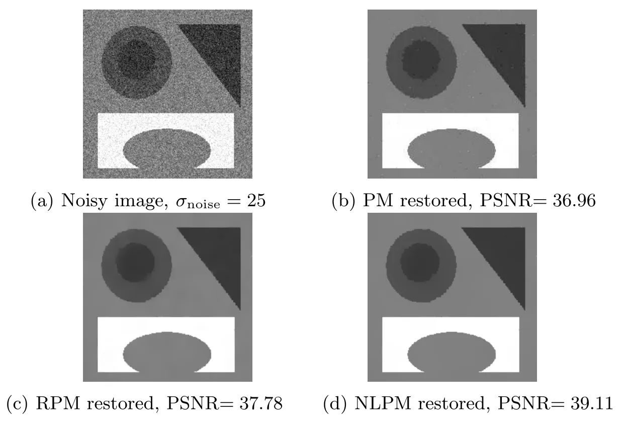
Figure 6 Restored results of three different diffusion methods

Figure 7 Detailed comparisons of restored images by the PM method and the NLPM method

Figure 8 Detailed comparisons of restored images by the RPM method and the NLPM method

Our next examples compare the performance of the proposed NLPM method with more PDE-based image denoising methods,namely,the total variation method (TV) [1],the PM method,the RPM method,the mild regularized PM method (M-RPM) [21],and the adaptive PM method (we use the same notation “D-α-PM” as the original article [30]).All of the parameters are chosen to be optimal based on the corresponding articles,also,the iteration is stopped when maximal PSNR value is reached.The best PSNR results of these six different PDE-based methods are listed in Table 2,and the test images are chosen from Figure 5.The highest PSNR value of each experiment is shown in bold face.For various types of images,our NLPM method demonstrates the best denoising ability among these six PDE-based methods.

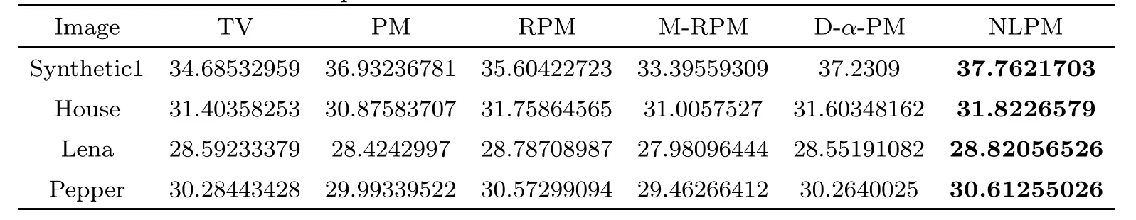
Table 2 The optimal PSNR results of different PDE-based methods

The visual results are presented in Figures 9–12,with the original image,the noisy image contaminated by additive Gaussian noise,and the images denoised by different methods shown in the respective subfigures.One notices that there are several random black and white speckles appearing in the images denoised by the PM method;that is because of the forward-backward diffusion.The RPM method loses the preservation of edge lines (such as the junction lines of the four squares in Figure 9(e)),due to the high regularization of its solutions.In the smooth intensity transition areas (such as the first three quadrants of “Synthetic 1” in Figure 9(a),the cheeks of “Lena” in Figure 11(a),and the smooth surface of “Pepper” in Figure 12(a)),the TV method has an obvious “staircase” effect as shown in Figures 9(c),11(c),and 12(c),while the M-RPM method exposes a more serious “staircase” effect in the corresponding experiments,demonstrated especially in Figure 9(f).This is because the M-RPM method depends too much on the parameterpin terms of its diffusivity (1.3),and the fixed parameterpresults in a lack of flexibility regarding its diffusion process.The D-α-PM method,specifically,

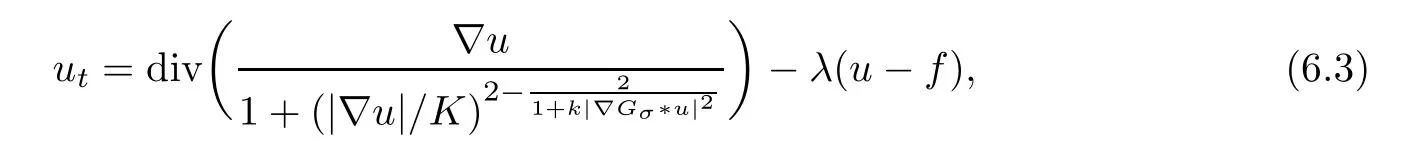
adopts an adaptive diffusivity which can effectively improve the drawbacks of the M-RPM method (as shown in Figures 9(g),11(g) and 12(g)).However,the D-α-PM method has too many parameters (namely,K,k,σ,λin (6.3),the time stepτ,and the iteration times) to modify,which increases the difficulty of implementation and limits the application of the Dα-PM method.Our NLPM method prevents the shortcomings mentioned above.Specifically,the NLPM method preserves the edges well (Figures 9(g) and 10(h)),restores the smooth transitions well,and avoids the “staircase” artifacts (Figures 9(h),11(h) and (12)(h)).It also presents visual effects as good as the D-α-PM method while having less parameters to modify.

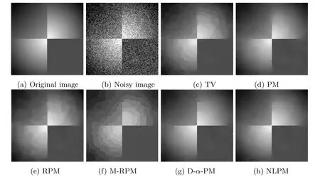
Figure 9 Experiments on “Synthetic 1”,of size 128 × 128,the noise standard deviation being 30

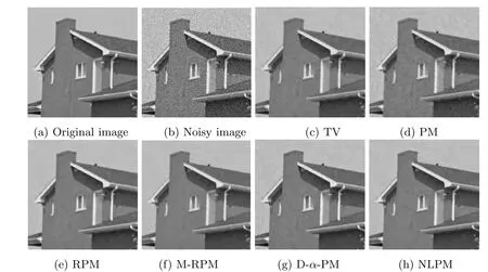
Figure 10 Experiments on “House”,of size 256 × 256,the noise standard deviation being 20

Figure 11 Experiments on “Lena”,of size 300 × 300,the noise standard deviation being 25

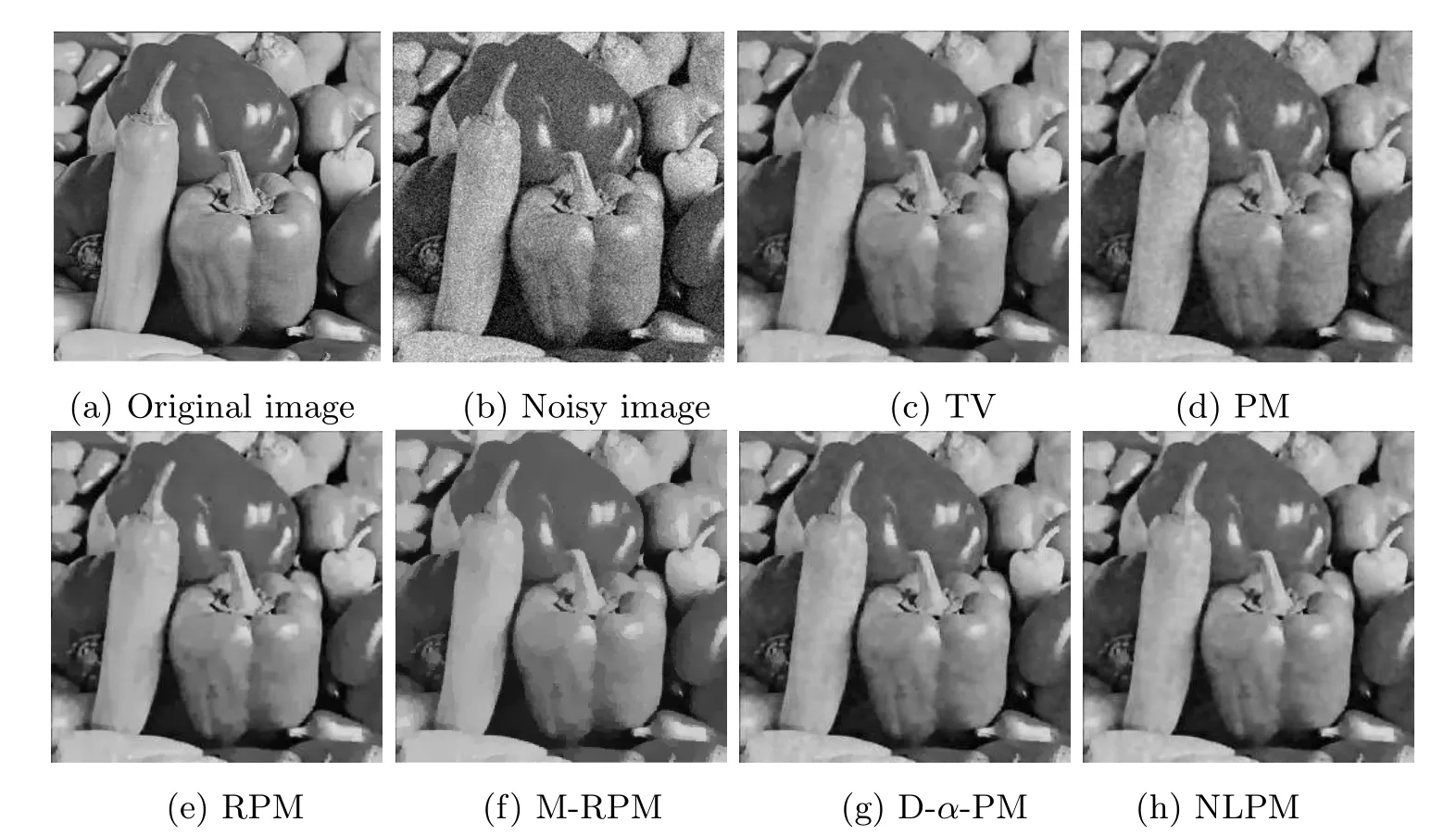
Figure 12 Experiments on “Pepper”,of size 256 × 256,the noise standard deviation being 20

6.3 Selection of Parameters

There are two main parameters,Kandσ,in our NLPM method that need to be modified in the experiments.

The parameterKis a threshold value of diffusion progress;it has more influence on the boundary and edge areas than the smooth areas.Consequently,there are differences of the optimalKamong different types of images.As for the images with fewer details,such as the“Synthetic 1” and “House” in Figures 9(a) and 10(a),the optimalKis smaller and lies between 3 and 5.For the images with more details,i.e.,the real natural images such as “Lena” and“Pepper” in Figures 11(a) and 12(a),the optimalKis supposed to be larger;around 7 -9.On the other hand,the noise level will also affect the optimal value ofK.Specifically,images with larger noise levels will have a larger optimalK,which is reasonable,since the noise will increase the “details” in the image.

The parameterσ,as discussed in Section 2,represents the non-locality level of diffusion progress.Throughout the experiments,we found thatσ=1 is an optimal choice for different types of images.On the other hand,to ensure the numerical stability of the PMS scheme,the time stepτis required to be less than 0.25.Also,according to our empirical evidence,the PSNR result will not increase afterτgets small enough.Therefore,we chooseτ=0.02 for all experiments to both satisfy the stability requirements and preserve the time efficiency.Finally,for the number of iteration times,we apply the maximal PSNR criterion,i.e.,stop the iteration when the maximal PSNR is reached.Therefore,the number of iteration times is fixed if all of the other parameters are given.In general,the number of iteration times is in proportion to noise level,and is inversely proportional toK.