
Pitman–Yor process mixture model for community structure exploration considering latent interaction patterns?
2021-12-22 06:47:26JingWang王晶andKanLi李侃
Chinese Physics B 2021年12期
關(guān)鍵詞:王晶
Jing Wang(王晶) and Kan Li(李侃)
School of Computer Science,Beijing Institute of Technology,Beijing 100088,China
Keywords: community detection,interaction pattern,Pitman–Yor process,Markov chain Monte–Carlo
1. Introduction
The modern world is highly connected through various interactions that form a large amount of complex networks containing huge valuable data.[1]There are amounts of important applications in the field of complex network, such as the identify influential nodes (Ref. [2]) predicting the evolution of collaboration(Ref.[3]), mitigating the spread of accidents(Ref. [4]) and optimizing the traffic in networks (Ref. [5]).One of the most popular topics of complex networks is the community structure, that is, the vertices divided into groups(also called clusters or blocks)on the basis of a specific criterion or measure.[6]
Newman and Girvan’s studies about social and biological networks show that the communities hidden in those datasets are composed of densely connected (or assortative)vertices, while are sparsely connected to those in different communities.[7,8]We call this type of communities with a higher inner connectivity assortative community. Definition of assortative community is ill-suited to the bipartite networks in which the vertices of same type are never connected,e.g.,user-item networks,author-paper networks and affiliation networks.[9,10]So in order to group one type of vertices in a bipartite network,we should resort to the methods different from those for the assortative community.[11]For simplicity,we call the communities in bipartite networks bipartite community.Besides, there exists other community structure in which the links are established less frequently inside the communities than those between the different communities,e.g.,transcriptional regulatory networks, shareholding networks, and cooccurring word networks.[12,13]We call the communities with higher external connectivity disassortative community.The diverse community structures bring about numerous community detection methods.
However,most existing methods and models focus on detecting certain types of community structures.[14–18]The methods that cannot explore the diverse community structures may fail or lead to biased results, if the network data becomes so complex that we cannot presume a prior for its community structures according to the realistic metadata(e.g.,vertices’or interactions’attributes)or the empirical studies(e.g.,relevant work).[19]Even though we can presume one type of community structure for a network,it is still possible that other types of community structures are hidden in the network. Therefore what we aim to design is a method that can automatically detect the types of community structures including the number of communities,community sizes and explainable vertexpartitions(see Fig.1).
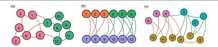
Fig. 1. The toy example of community structure exploration. A competent model should detect three diverse community structures. The colors of vertices represent the different communities found by a community detection method. The colors of links represent the different interaction patterns. (a)Assortative communities;(b)bipartite communities;(c)disassortative communities.

Fig.2.A toy example of relations between the density of interactions and the vertex partitions:the vertices of the same color own similar interaction patterns. If the interactions are removed,the interaction patterns may alter and so do the vertex partitions. (a)Network of 32 vertices and 89 edges;(b)network of 32 vertices and 71 edges;(c)network of 32 vertices and 53 edges.
One of the most used, flexible and powerful statistical models is the stochastic block models(SBM).[20]It can characterize the assortative community, bipartite community and even disassortative community.[6]There are numerous variants based on SBM or modified SBM,for instance,for the assortative community,[21,22]the bipartite community[10,23]and even the disassortative community.[13]However,in order to achieve a higher likelihood in the parameter inference process, the methods based on the SBM are prone to divide a community even if the vertices in this community have similar behaviors.[24]This character sometimes leads to meaningless and unexplainable results. For instance, a group of peopleAbuy itemsC,D, andEwith high probabilities, while another group of peopleBbuy itemsC,D, andFwith similar probabilities. To prevent overfitting,it is more reasonable to merge these two groups into one community because of similar purchasing habits. This paper will propose an approach to cope with this kind of overfitting.
Community structures can refer to groups of vertices that connect similarly to the rest of the network.[25]Following this idea, we propose an innovative way of defining a community,i.e.,incorporating the interaction pattern into community structure, that is to say, all vertices in the same community should share a property in common and the property determines how the vertices interact with the rest of the network.Under the diverse interaction patterns,different types of community structures can be easily represented. Furthermore,the interaction patterns can help our model avoid the kind of overfitting introduced above and lead to explainable results. In this definition,the interactions or links are regarded as statistical units and evidence. The latent interaction patterns will be learned automatically by our model according to the evidence from network data. Specifically,when the interaction patterns are weak,the statistical evidence will be less likely to support grouping the vertices into the same community,and vice versa(for illustration see Fig. 2). The interaction patterns also can be regarded as the features of the communities. But the community exploration through statistical models differs from data classification by feature selection.[26]Our model aims to learn the latent and unknown features described by our assumption,
whereas feature selection for data classification aims to learn a subset of features that have already been given.
We then propose a Pitman–Yor process mixture model subtly incorporating interaction pattern in communitystructure exploration. Under the rule of the Pitman–Yor process, it can automatically discover reasonable numbers and sizes of communities without any extra information about the community structures and the conversion or projection of the adjacency matrix.Besides,it also can estimate interaction patterns by utilizing Bayesian inference based on the revealed network structure, which offer more information for network analysis. Moreover, experiments have been conducted covering three types of community structures.
Our contributions are summarized as follows:
1. We propose a flexible and effective Pitman–Yor process mixture model inventively incorporating the interaction pattern. It can automatically discover the explainable community structures,even if the interactions are complex.
2. We propose a full-featured collapsed Gibbs sampling inference for community structure exploration. Not only can it lead to an explainable result but also estimate the latent interaction patterns through Bayesian inference.
3. Detailed experiments with visualizations on 11 real networks of different community structures prove that our model can efficiently reveal complex hidden interactionpatterns and outperforms the state-of-the-art SBMbased models.
2. Related work
The majority of existing approaches are designed for only one type of community structure. For instance, the methods based on random walk for assortative community,[18]the spectral methods for assortative community[16]and for bipartite community,[14]the optimization methods for assortative community,[17]bipartite community,[9]and both of them,[26]the methods based on statistical inference for assortative community[21,22,24,25]and bipartite community,[23]and the deep learning methods for assortative community.[28,29]To adapt one approach for another community structure considerable work is needed. For example, Newman proposed the original modularity to measure assortative community,[30]but it should be modified to be the bipartite modularity for the bipartite community.[9,14]Some other approaches are designed for multiple community structures,[13,27]but they suffer from resolution limit. The approaches based on statistical models employ a principled set of tools for community detection tasks.[6]They can be easily extended to fit the different community structures.[13,23]In this paper,we focus mainly on the statistical models.
One of the most significant statistical models for community detection is the stochastic block model (SBM).[20]Although the SBM has been extensively studied, there still have been numbers of novel approaches based on it in recent years.[22,25,31,32]The block adjacency matrix is a pivotal assumption in the standard SBM. The elements in this matrix define the connection probabilities between two blocks or within a block.[21]To apply statistical inference, each vertex should be assigned to only one block which just corresponds to a community this vertex belongs to. The connection probabilities between two vertices only depend on their blocks,i.e., communities.[21]Different choices of connection probabilities in a block adjacency matrix can lead to different community structures, such as assortative community structure,bipartite community structure, and disassortative community structure.[6]
However, the standard SBM faces two open challenges.Firstly, due to the model’s assumption, all vertices within the same community have the same degree distribution, which makes the nodes with the same degree be probably assigned into the same community.[31]The degree-corrected stochastic block model(DCSBM)proposed by Karrer and Newman offers one way to accommodate the degree heterogeneity and allow the vertices of varying degrees to be grouped into one community.[22,33]Because of the broader degree distribution in the communities, DCSBM becomes a widely used generalization of SBM. However, for some networks, DCSBM tends to divide groups even if the group of vertices have similar behaviors. This action can increase the density of links in one block or between two blocks but sometimes may lead to overfitting. Another novel statistical method is the completely random measure stochastic block model(CRMSBM),which incorporates the mass or sociability (similar to degree correction)of vertices and block structure into the completely random measure.[34]However,the number of communities inferred by CRMSBM is closely related to the initial number of communities,which causes CRMSBM unstable performances on some datasets. We will show it in Subsection 4.2.
The second challenge is that the standard SBM requires a specific number of groupsKas a prior in order to apply inference. However,Kusually varies according to different community structures,network scales and research areas. Using a model selection criterion is one approach to decide whichKto choose, e.g., minimum description length (MDL).[35]Regarding the number of groups as a parameter of the model and selectingKdirectly from the Bayesian inference process is another approach. For instance, use approximate inference, i.e., Markov chain Monte–Carlo (MCMC) to sample community assignments of vertices according to the posterior distribution,[32]or use Bayesian nonparametric models to let the model decide whichK(the complexity of the model)to choose, e.g., Chinese restaurant process (CRP) combined with SBM[36,37]and CRP combined with DCSBM.[38]Deep learning for community detection is developing rapidly in recent years.Its powerful feature-representation ability offers us other opportunities to detect community structures by extracting vertices’ features.[28]The deep generative latent feature relational model (DGLFRM) proposed by Mehta (Ref. [29])combines the advantages of variational graph autoencoder and the SBM. It can learn the strength of latent memberships for each vertex and the number of communities can also be learned by the sparse membership representation. However,because of the vague definition of community and unexplainable embedding space,the memberships of the vertices cannot represent the community assignments.
Even though considering the degree correction or the Bayesian nonparametric as a prior or learning the latent membership makes the standard SBM capture various types of community structures,[37]the block that has denser links is just one way to produce communities. As a more general perspective in Abbe’s review,[25]community structures can refer to clusters of vertices that connect similarly to the rest of the networks. In this paper, the interaction pattern we proposed is just corresponding to the above viewpoint and makes our model characterize the three types of community structures or even the mixture of them. In addition,the modeling of degree heterogeneity is also allowed under the assumption of the latent interaction pattern. We will let the inference algorithm choose the numbers and sizes of communities just like these articles(Refs.[37,38]). But we consider the extension of CRP as prior, i.e., the Pitman–Yor process (PYP), which can offer a reasonable community size distribution when the number of communities becomes large.[39]
We next formulate our model specifically and derive an inference algorithm.
3. Model and inference
The notations used in this paper are summarized in Table 1. We use the terms interaction,link and edge interchangeably,and the terms vertex and node interchangeably.

Table 1. Notations frequently used in this paper.
3.1. Model
In this paper, a set of interactionsXn?{Xi}iconstitute the network data,wherei=1,...,n.The interactionXi=(r,s)is represented with two endpoints,vertexrands.
3.1.1. Interaction pattern
Firstly,as we introduce briefly in Section 1,we consider the variables describing the interaction patterns and how these variables are accommodated to community structures. We assume that the generation of an interactionXi=(r,s) can be divided into two steps. Firstly, a vertexrstarts the head of an interactionXi, then another vertexsaccepts the tail of the interactionXi. This process can be simply illustrated by a purchasing process in which,for example,a customer selects cereals out of fruits, bread and sandwiches for breakfast. The interaction will be started by the customer as the interaction’s head. Next,the prices and the flavors of the cereals will affect the customer’s decision. Then a certain cereal product finally“accept”this interaction as its tail. This process can result in the emergence of interaction patterns,say a probability vectorη,with which the customer chooses diverse goods.
Secondly, we assume if the heads are in the same communityj,they have the same interaction pattern according to our way of defining the community. For instance, the customers in the communityjwill choose goods with probability vectorηj?. Specifically,the probability vectorηj?=(ηjs)sdenotes the interaction pattern hidden in the communityj,wherej ∈(1,...,k) denotes a unique community in allkcommunity, ands ∈(1,...,l) denotes a unique vertex in the vertex set. The vectorηj?is normalized, i.e., ∑s ηjs=1. Different communities will have differentηj?. Just like in the purchasing process,different types of customers will choose the food for breakfast with different interaction patternsηj?. This definition of interaction patternηj?can characterize diverse community structures including assortative community, bipartite community and disassortative community. We prove that as follows.
Letφj1j2denotes the probability of an interaction between two vertices belonging to the communityj1andj2respectively. Actually,φj1j2is the same as the elements of the block adjacency matrix in the standard SBM.From the definition ofηjswe can get
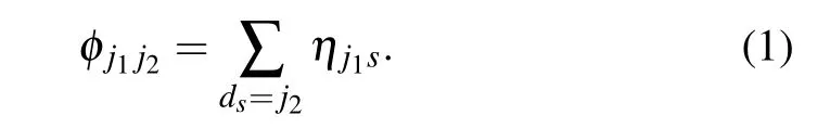
Apparently, the link patternηj?can represent all the connection probabilities between two blocks and in a block, which parameterizes SBMs. This interaction-pattern definition is also suitable for both directed and undirected networks. An undirected interaction can be divided into two opposite headto-tail interactions, which means both endpoints of this interaction will accept the head-to-tail link started by another endpoint.
The parameters discussed above characterize the interaction patterns and their relations with communities. Furthermore,we need a prior for the community-assignment process of vertices. The community-assignment can be considered as a random sequenceDl?(D1,...,Dl) that consists of a sequence of positive integers,in which the elements indicate the community a vertex belongs to. This random sequence can also be viewed as a random partition produced by the Pitman–Yor process (PYP).[39]The one-parameter simplified form,i.e., Chinese restaurant process (CRP), has previously been used to determine the numbers and sizes of communities in other SBMs.[36,38]As far as our knowledge, PYP has seldom been employed by the existing community detection methods.Furthermore,the Bayesian nonparametrics including PYP and CRP are flexible and effective priors to represent the community partitions with different numbers and sizes,and also make the inference process easy to implement.[37]
3.1.2. PYP
The PYP is a two-parameter extension to the CRP,which allows heavier-tailed distributions over partitions.[40]PYP can be interpreted by a CRP metaphor in which the objects are customers in a restaurant, and the groups are the tables at which the customers sit.[41]Imagine a restaurant with infinite tables,each with a unique label. The customers enter the restaurant one after another and then choose an occupied table with probability proportional to the number of occupants minus a discount parameterθor choose a new vacant table with probability proportional to the concentration parameterαplusk×θ,
wherekis the total number of occupied tables. When the discount parameterθequals to 0, the PYP becomes the CRP.Usually,the PYP and the CRP is used as a prior in the mixture model with an infinite number of latent components,but a finite number of them are used to generate the observed data.[42]In this paper, each community represents a latent component and the interactions are generated according to the interaction patterns associated with the communities of their heads.Compared to the CRP metaphor,the tables denote the communities,a customer denotes the head of an interaction, and the latent components denote the latent interaction patterns. When the(n+1)-th customer enters the restaurant withncustomers andkoccupied tables,the new customer will sit at the tableior a new table with the probability as follows:

wherecidenotes the number of customers at the tablei.
3.1.3. Generative process
The generative process for an interaction setXn,ηj?andDlcan be constructed as follows.
1. Choose a headrof an interaction uniformly with replacement from a finite vertex setVl.
2. Assignrto a communitydraccording to PYP with the concentration parameterαand discount parameterθ.
3. If the community ofris previously occupied,go to the next step,or if the community is new,draw a probability vectorηdr?for this cluster according to a symmetric Dirichlet distribution with parameterβ. In order to generalize our model to fit various interaction patterns, we choose a mild prior,i.e.,a symmetric Dirichlet distribution.
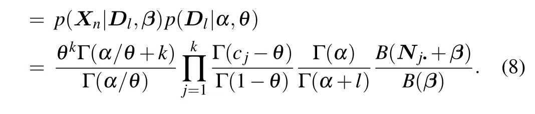
4. Then the headrestablishes a link to the tailsaccording toηdr?.The joint probability induced from the above generative process can be written as
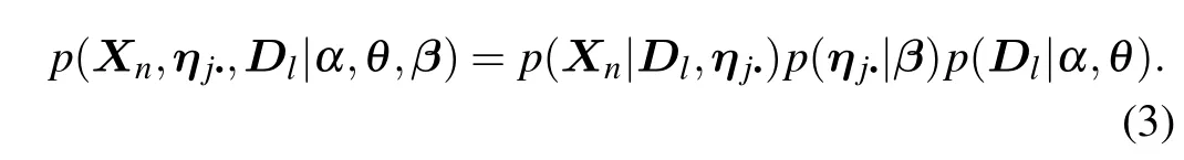
The three factors on the right side can be written as

whereNjsdenotes the number of tails from blockjtos.
Given the observation ofXn, the Bayesian inference framework can be used to estimate the unknown parameters.To be brief,we call our model“PYP-IP”(Pitman–Yor process mixture model considering latent interaction pattern).
3.2. Inference and estimation
3.2.1. Parameter and hyperparameter inference
Because the exact inference on two multivariate random variablesηj?andDlis intractable,we employ a Markov chain Monte–Carlo(MCMC)algorithm for an approximate estimation. Then the interaction patterns can be estimated through the discovered community structures.kmay vary according to differentDlinference onηj?. In addition,the dimension ofηj?will grow along with the number of vertices. It results in a rapid expansion of the sample space ofηj?along with the network size. So tremendous samples are required to reduce the estimation error. With the help of the conjugacy between the Dirichlet and multinomial distributions, we can simplify the joint distribution of the first(Eq.(6))and the second(Eq.(5))factor in Eq.(3).
GivenDlandβand letηj?~Dirichlet(β),the joint probability ofXnis as follows:
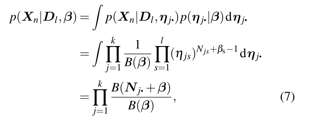
whereNj?denotes a vector containingNjsin Eq. (6). After integrating outηj?,we obtain the likelihood

Another multivariate random variableDlrepresents the latent community assignment. They can be updated by Gibbs sampling scans(sweeps)in light of the CRP metaphor. A vertex labeldrcan be updated at each sampling move by fixing the remaining variables in the whole vectorDl, wherer ∈(1,...,l). So For the derivation of the posterior distribution of hyperparameters(formula(10)),it is highly recommended to refer to Teh’s article(Ref.[43]).
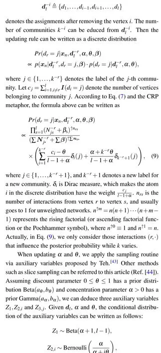
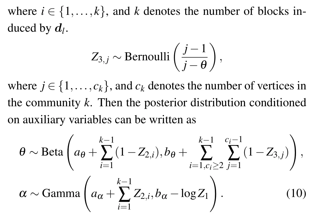
We can update another hyperparameterβsaccording to its fully conditional posterior. Becauseβsis independent ofαandθ,we can easily deduce the posterior distribution from Eq.(7)
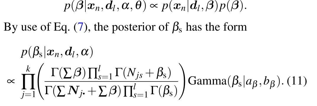
Then slice sampling can be applied to updateβs. One Gibbs scan or sweep of sampling process includes the updating steps defined in Eqs.(9)–(11),respectively.
Let hyperparametersα,βshave the prior Gamma(1,1)andθhas the prior Beta(1,1)to make the Bayesian inference algorithm automatically estimate these hyperparameters. In addition,the mild priors Gamma(1,1)and Beta(1,1)make the model flexible.
3.2.2. Estimation
Select the best partition. Although after enough iterations our MCMC algorithm can converge,for the analysis task it is still worth finding the best partition according to Bayesian model comparison. Given the observationXn, we can select the best partition by calculating the posterior probability of all the parameters in the model
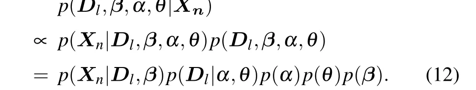
This posterior probability can be calculated according to Eqs.(4)and(7).
Estimation of interaction pattern After applying the MCMC sampling above, we can obtain the estimated community assignments ?dlfor all the vertices. Simultaneously,the hyperparameters, i.e.,α,θ, andβare estimated, which describe the interaction patterns of the model. Given all these estimated parameters and the training dataxn, we apply Bayesian inference for the posterior estimation of the interaction pattern ?ηjs, wherej ∈{1,...,?k}. The estimation of ?ηjsequals to the posterior predictive distribution of a link ?x=(r,s),where the vertexrbelongs to the communityj.
We first give the prediction rule for a new link. Given an unobserved interaction ?x=(r,s), we can estimate the probability of this link according to
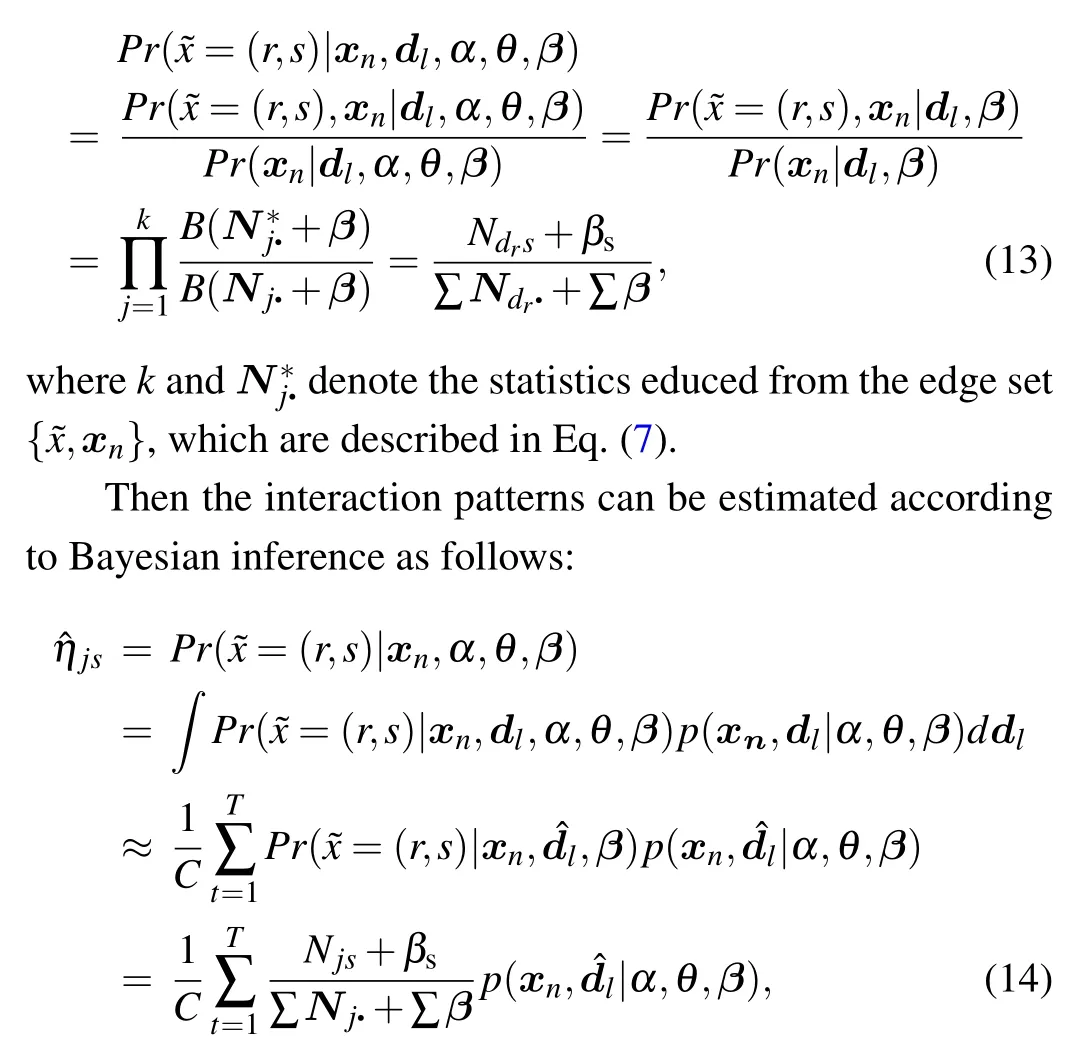
where{Nj?}jdenotes the statistics educed from the edge setxnand ?dl, which are described in Eq. (7), andTdenotes the number of iterations after the burn-in period. The normalization coefficientCequals to ∑Tt=1p(xn,?dl|α,θ,β), which can be calculated via Eq.(8).
3.2.3. Time complexity
The time complexity of our algorithm mainly depends on the MCMC sampler. The runtime per MCMC iteration largely depends on the Gibbs sampling scan forDl(Eq.(9)). So we can estimate the total runtime asT=O(?KLNit), where ?Kis the estimation ofK,Lis the number of vertices, andNitis the iteration times. The function of drawing samples from a discrete distribution(described in Eq.(9))is the essential step of MCMC sampling. The different realization of this function will impact on the runtime notably. So the code optimization for this function can improve the running speed significantly.
4. Experiments and results
4.1. Datasets
Here we apply PYP-IP to the undirected network data of different sizes,types and community structures. Experiments are run on eleven datasets,i.e.,characters’co-occurrence network in Les Miserables (Les Mis), the “core” of the email-EuAll network (Eu-core), the protein-protein interaction network in yeasts (Yeast) scientific publication citation network(Cora),the network of hyperlinks between weblogs on US politics(Poli blog),attendance at 14 social events by 18 Southern women (Wom-eve), human musculoskeletal network (Musske), the network denotes which languages are spoken in which countries (Coun-lang), over 100k ratings from Movie-Lens datasets(ML-100k), adjective-noun word network(Adjnoun), and human transcriptional regulatory network (Tranreg).
The details of the datasets are shown in Table 2.
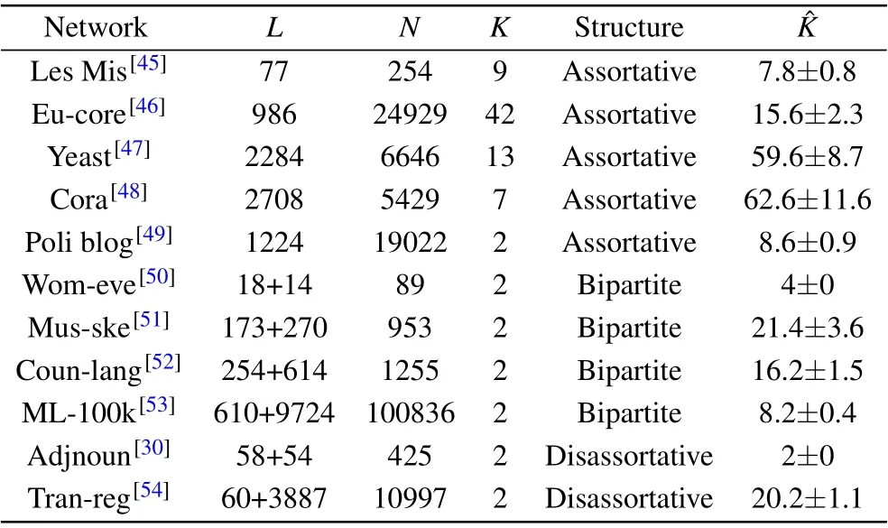
Table 2. Dataset details and estimated block numbers.
Self-interactions exist in real network data, such as selfhyperlink and emails to oneself. According to the definition of interaction pattern, a vertex can interact with itself with some probability. So self-loops are allowed in our model. We eliminate self-loops and the isolated vertices for comparison with other models, so that the number of vertices and interactions may be different from the original datasets (include Eu-core, Yeast, Poli blog, ML-100k and Tran-reg). The data pre-processes and the MCMC sampler are implemented by R language and Matlab(R),respectively. All the code are run on a workstation(Intel(R)Xeon(R)CPU E5-2640 v4@2.40 GHz with 64 GB memory).
4.2. Community structure exploration
Community structure exploration can give us some insight into the seemingly disorganized networks. The consideration of interaction pattern makes PYP-IP capable of discovering the latent link patterns.
We apply PYP-IP to group the vertices in the realworld networks without knowing the types of community structures and the number of communities beforehand, to check if PYP-IP can detect the correct community structures. For a fair comparison, all the models in experiments should detect the numbers and sizes of communities automatically. PYP-IP is compared against the infinite relational model (IRM) inferred via Gibbs sampling,[37]the DCSBM inferred via Metropolis–Hastings sampling with joint mergesplit moves,[32]the CRMSBM inferred via Gibbs sampling and Metropolis–Hastings sampling together,[34]and DGLFRM based on variational graph autoencoder combined with SBM.[29]For all the models, the network data will be treated as a square adjacency matrix and all the models do not use any prior information about community structures,such as the number or the sizes of communities. The number of communitiesKwill be initialized by randomly sampling from 1 to log(L). Given the number of communitiesK,the community assignments of all vertices will be also initialized randomly.For a fair comparison, DGLFRM will learn the membership of each vertex without extra vertex attributes and each vertex is assigned to the community that has the maximal strength of its community membership. The parameter settings of IRM,DCSBM,CRMSBM and DGLFRM are default as the authors’codes(thanks to these authors generously offering their codes online).
The iteration times of our MCMC sampling are set from 200 to 1000 according to the size of the datasets.All the scores are averaged over 10 restarts.
4.2.1. Assortative community detection
The experiments on the 5 datasets exhibiting assortative community structure will check the models’ stability and validity in detecting the densely connected groups. The normalized mutual information (NMI) is used to measure the correlation between clustering resultsd′lwith the ground truthdl.NMI is calculated as follows:
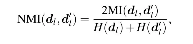
where MI(dl,d′l)is mutual information andH(dl)is entropy ofdl. The results are shown in Table 3 with their means and standard variances.

Table 3. NMI score of the clustering results multiplied by 100 with their standard variances. All scores are averaged over 10 restarts.
For assortative community structure,the results show that PYP-IP surpasses the other four models. The performances of all models drop on “Yeast” and “Cora” mainly because of sparser interactions than other networks. DCSBM with joint merge-split moves outperforms IRM and CRMSBM.Both the degree correction and the merge-split moves contribute to the performance of DCSBM.CRMSBM has larger standard variances on“Les Mis”,“Cora”,and“Poli blog”,which shows it is not as stable as the other 4 models. The number of communities discovered by CRMSBM is closely related to the initial number, which causes the unstable performances. Although DGLFRM can learn the latent membership of vertices and the number of communities,sometimes the unexplainable embedding representations are hard to capture community structures.
4.2.2. Bipartite community detection
Bipartite networks have two types of vertices, i.e., the type I and type II, so we assume there are at least two basic communities in bipartite networks. The bipartite community is quite different from the assortative community,that is,there are no interactions within any communities. So models for bipartite community exploration should have two essential functions: 1) distinguish vertices between two types(two basic communities), and 2) group the vertices into the sub-communities. If a model can achieve the first function,the interactions between the bipartite communities should always be detected between two different communities (external links), no matter how the model group the vertices into the sub-communities (see Fig. 1(b)), e.g., woman-event links and person-corporation links should always happen between communities.
Therefore,let the F1 score(F1)help us examine whether the model can achieve the first function. For bipartite community detection,if an interaction is recognized as an external one when the ground truth is external,this sample is true positive(tp),and if an interaction is recognized as an internal one when the ground truth is external,this sample is false negative(fn). F1 score is calculated as follows:

where“fp”stands for false positive. However,if we exchange the community assignments of a link’s head and tail in bipartite networks, the corresponding links may still be external whereas the partition error rate will increase. Here we employ another metric,partition error rate(PER),to measure the partition results for bipartite networks. If a vertex from type I is assigned to type II, PER will increase. It is calculated as follows:

where“#()”stands for the number of something.
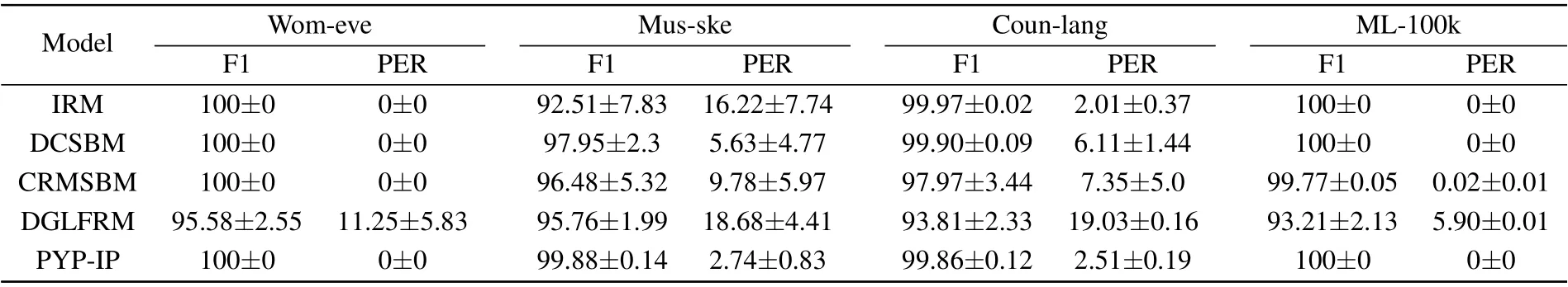
Table 4. The F1 scores and PER of the clustering results multiplied by 100 with their standard variances. All scores are averaged over 10 restarts.
The F1 scores and PERs of bipartite community detection are shown in Table 4 with their means and standard variances.The four datasets of bipartite networks do not have the groundtruth of sub-community structure. According to that paper,[19]we just use the types of nodes as the ground truth. So all the bipartite networks haveK=2.
The results show that four statistical models have the ability to automatically detect the bipartite communities on the four datasets. The DCSBM has a higher F1 score and a lower PER on “Coun-lang”, whereas PYP-IP has the opposite results. In this situation, we will evaluate the models by PER.Because DCSBM is more likely to exchange the community assignments of vertices in”Coun-lang”,which makes some interactions are still external. DGLFRM can detect the external interactions in bipartite networks,but assigns more frequently the two endpoints of interactions to the incorrect vertex type.So its PERs increase a lot.
According to the second function, a model may further split the two basic communities into sub-communities based on the different criteria, e.g., the women attending similar events,i.e.,the vertices’behaviors(“Wom-eve”see Fig.6(b))or e.g.,the collaborative relationship between muscles,i.e.,the vertices’ functions (“Mus-ske” see Fig. 11(b)). This split by PYP-IP is based on whether the communities have similar interaction patterns and can reveal the latent interaction-pattern information(shown in Subsection 4.4)that is meaningful and explainable.
Although “ML-100k” (99.81% sparsity) is sparser (as normal or square adjacency matrix)than“Mus-ske”(99.03%sparsity), the results (F1 score and PER) are better for “ML-100k” than “Mus-ske”, because “ML-100k” contains more interaction-pattern evidence than“Mus-ske”if we regard their network data as the bipartite or rectangular matrices (a user had rated at least 20 movies, but a bone is connected to an average of 5.5 muscles). This result is consistent with our reasonable assumption depicted in Fig.2.
4.2.3. Disassortative community detection
Because both of the datasets have two types of vertices and this condition is similar to bipartite networks,we can also use the F1 score and partition error rate(PER)to examine the exploration result. In“Adjnoun”dataset,some adjectives can be connected to other adjectives,and some nouns can be connected to other nouns. In“Tran-reg”dataset, some transcription factors not only regulate the target genes but also regulate other transcription factors. So the main difference between disassortative communities and bipartite communities is that the former can have internal interactions,but the later cannot.The F1 scores and PERs of the disassortative community detection are shown in Table 5 with their means and standard variances.
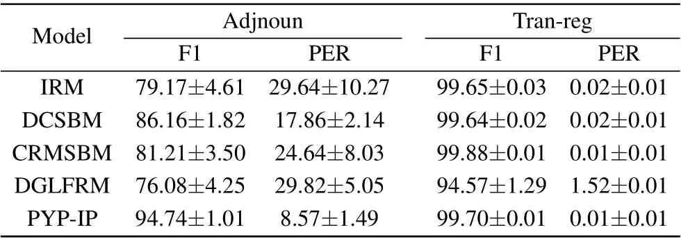
Table 5. The F1 scores and PER of the clustering results multiplied by 100 with their standard variances. All scores are averaged over 10 restarts.
Although both“Adjnoun”and“Tran-reg”have the disassortative community structure, all five models’ performances on “Adjnoun” drop more. That is because the percentage of the internal interactions within two communities in“Adjnoun”(38.9%) is significantly larger than in “Tran-reg” (0.86%).However, PYP-IP performs much better than the other four competitors and nearly recovers the disassortative community structure of“Adjnoun”(see Fig.5(d)).
4.3. Other results
MCMC Convergence. We run our MCMC algorithm on four datasets “Yeast”, “Cora” “Adjnoun” and “Mus-ske” to check the convergence of MCMC. Log-likelihoods (Eq. (8))are recorded as they-axis and the numbers of iterations are recorded as thex-axis. The results are shown in Fig.3.
The algorithm can reach the high-probability area of the likelihood for the four datasets with different community structures. When the dataset becomes sparser,e.g.,“Mus-ske”99.03% sparsity and “Cora” 99.85% sparsity, the algorithm needs more iterations to convergence. We will analyze it in the next paragraph.
Hyperparameterβ.βis very important to PYP-IP. Its value will go larger when the networks are denser and have more internal interactions. Its value will go smaller when the networks are sparser and have more external interactions. For example, “Adjnoun” is denser and has more internal interactions,so it has the largeβs. The box plot ofβsfor the datasets is shown in Fig.4.
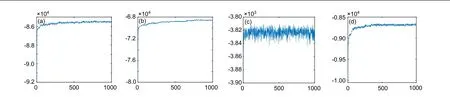
Fig.3. Log-likelihood after each MCMC iteration. (a)“Yeast”;(b)“Cora”;(c)“Adjnoun”;(d)“Mus-ske”.
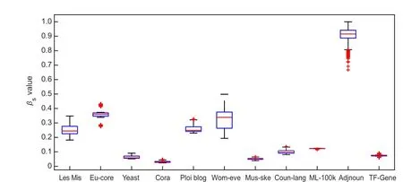
Fig.4. Box plot for βs. We keep βs values of the last 500 MCMC iterations at each of 10 restarts. There are 5000 values in total for each dataset.
Sparsity and community size. PYP-IP inclines to estimate a larger ?Kand group the vertices into smaller communities when the networks are sparser(refer to Table 2). Because usually there is not enough evidence to support merging the vertices into a larger community in sparse networks. But if there is more interaction pattern evidence, our model tries to group the vertices that have similar latent interaction-patterns into the same community(see Figs.5(b)and 6(d)). This character offers reasonable vertex partitions for PYP-IP and it is consistent with our assumption illustrated in Fig.2. The IRM and DCSBM have similar characters, that is, when the networks are sparser the number of blocks increases so that the density of links in a block or between two blocks increases(refer to Fig. 12). The CRMSBM will infer the number of communities closely related to the initialized number and lead to the unstable performances(see Table 3).
4.4. Visualization
After the community structure exploration, we visualize the clustered networks to check if PYP-IP can explore the hidden interaction-patterns,which will offer extra information for link analysis. The adjacency matrices of networks are showed by rearranging the vertices according to the clustering results.The colored bars on the top and left stand for different communities,which are ordered by community sizes. The vertices in the communities are ordered by their degrees. Parts(a)and(c) of Figs. 5 and 6 show the ground-truth communities, and Part(b)and(d)of these figures show the clustering results by PYP-IP.
Figure 5(b) shows PYP-IP can find a latent link pattern that is a group of vertices having a distinct interaction behavior. These vertices are contacted by other vertices in different communities with higher probabilities than those in other communities. Figure 5(d)shows PYP-IP can detect the interaction patterns that are hidden in “Adjnoun” network, while IRM,DCSBM,and CRMSBM fail to do that. These interaction patterns explored by PYP-IP are not only meaningful but also beneficial to link analysis.
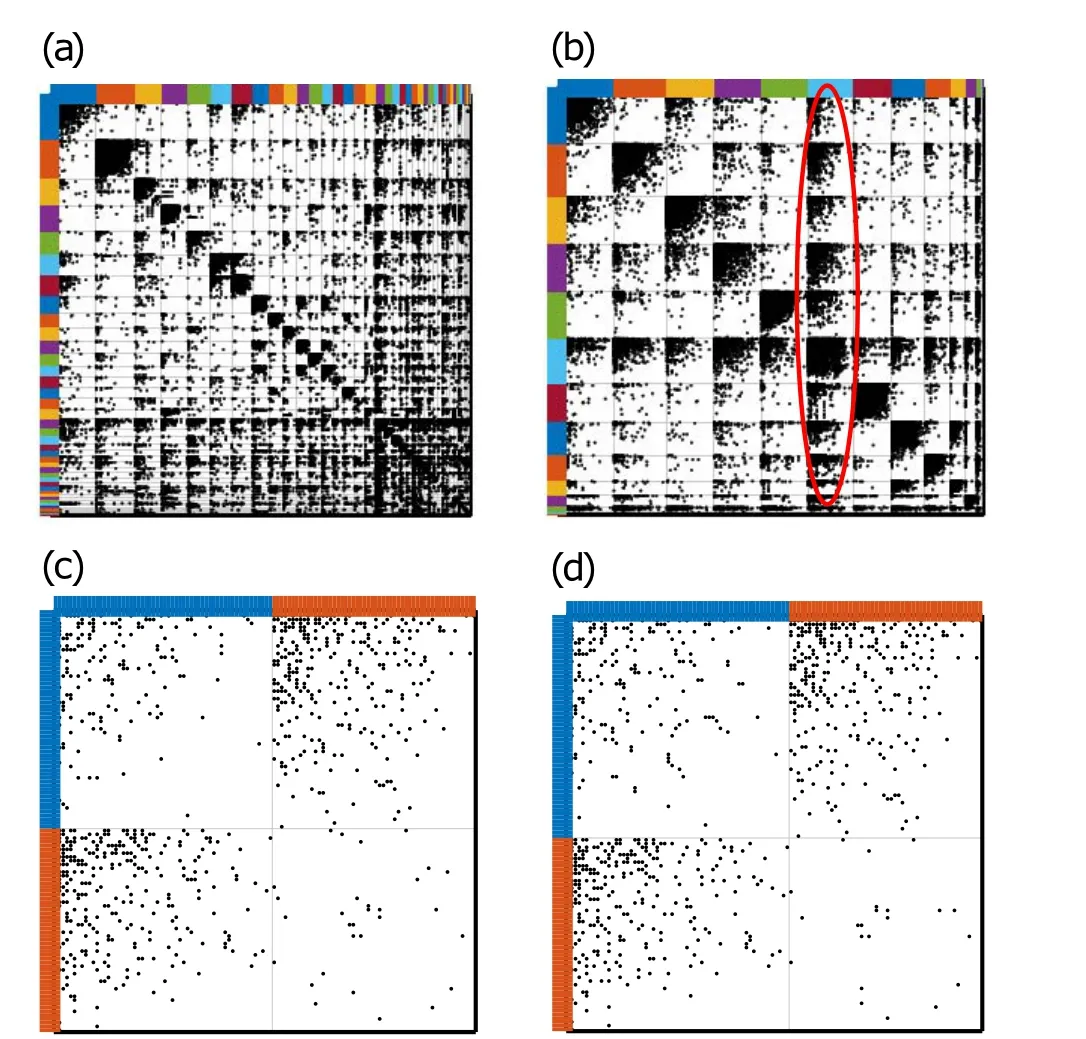
Fig. 5. (a) Ground-truth communities of “Eu-core”; (b) clustering results of“Eu-core”by PYP-IP:in assortative community structure, some distinct interaction-patterns are found. We first estimate ηjs by Eq. (13) and then calculate φj1 j2 by Eq.(1). The vertices in the red circled community(light blue community in (b)) are connected with a higher average probability(ˉφ·l =0.16, where “l(fā)” stands for the light blue community) than those in the purple community(ˉφ·p=0.09,where“p”stands for the purple community); (c) ground-truth communities of “Adjnoun”; (d) clustering results of“Adjnoun”PYP-IP:comparing(c)and(d), we find the disassortative communities in“Adjnoun”are almost recovered by PYP-IP,while the other comparative models have apparently higher partition error rates.
Figure 6(b)shows the women in orange and yellow communities attend some disjoint events. The two groups of women have the diverse social behaviors. Figure 6(d) shows the blog users’ different interaction patterns, that is, more communication with the others outside their community than those in other communities. Although the ground-truth shows the network (“Poli blog”) has assortative communities, there actually are “disassortative” communities hidden in assortative community structures. These diverse interaction patterns detected by PYP-IP will offer extra evidence compared to the original partition.

Fig.6. (a)Ground-truth communities of“Wom-eve”;(b)clustering results of“Wom-eve”by PYP-IP:according to attendance in disjoint events,18 women can be grouped into 2 communities(the blue and orange)corresponding to two groups of 14 events(the yellow and purple);(c)ground-truth communities of“Poli blog”; (d)clustering results of“Poli blog”by PYP-IP:we first estimate ηjs by Eq.(13)and then calculate φj1 j2 by Eq.(1).Although the ground truth shows“Poli blog”consists of assortative community structure,there actually is the disassortative community structure(red circle),that is,the users in the orange community interact more often with the yellow community(φoy=0.47,where“o”stands for the orange community and“y”stands for the yellow community)than their own community(φoo=0.32),and the users in the yellow community interact more often with the orange community(φyo=0.53)than their own community(φyy=0.33).

Fig. 7. Clustering results of “Tran-reg”: the same color in (a) and (b) represent the same community. In the disassortative community structure,the vertices of the same type can interact with others. From (a) and (b) , we can see in the disassortative community detection PYP-IP finishes two coupled jobs simultaneously: it detects the bipartite communities (a), meanwhile, one type of the vertices in which are grouped just like the assortative community detection (b). (a) Bipartite or rectangular matrix. Columns represent the transcription factors, rows represent the target genes;(b)interactions between the transcription factors.
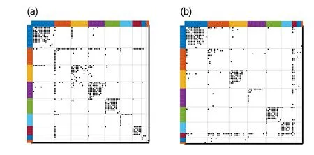
Fig.8. (a)Ground-truth communities of“Les Mis”;(b)clustering results of“Les Mis”by PYP-IP.
We do not visualize the square adjacency matrix of“Tranreg”, because most of the elements are blank(no interactions between“target genes”). Instead,we visualize the rectangular or bipartite adjacency matrix (x-axis andy-axis in Fig. 7(a)represent “transcription factors” and “target genes” respectively) and the square adjacency matrix of “transcription factors”(Fig.7(b)).
More results and figures are presented in Figs.8–11.Parts(a) of Figs. 8–11 show the ground-truth communities, and parts (b) of these figures show the clustering results of our model. These figures show that PYP-IP tries to group the vertices into smaller communities when the networks are sparse and do not have enough interaction-pattern information or evidence. Therefore,the communities are split into smaller ones.When the vertices have similar latent interaction-patterns,PYP-IP groups them into the same community. The following results are also consistent with the assumption proposed in Fig. 2. For some networks, the methods based on SBM such as DCSBM try to divide blocks into smaller ones so that the links in a block or between two blocks become denser (see Fig.12)and the likelihood becomes higher. However,the vertices that have similar link patterns are separated into different communities and then the link patterns fade away.
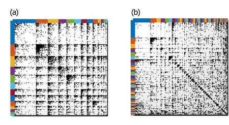
Fig. 9. (a) Ground-truth communities of “Yeast”; (b) clustering results of“Yeast”by PYP-IP.
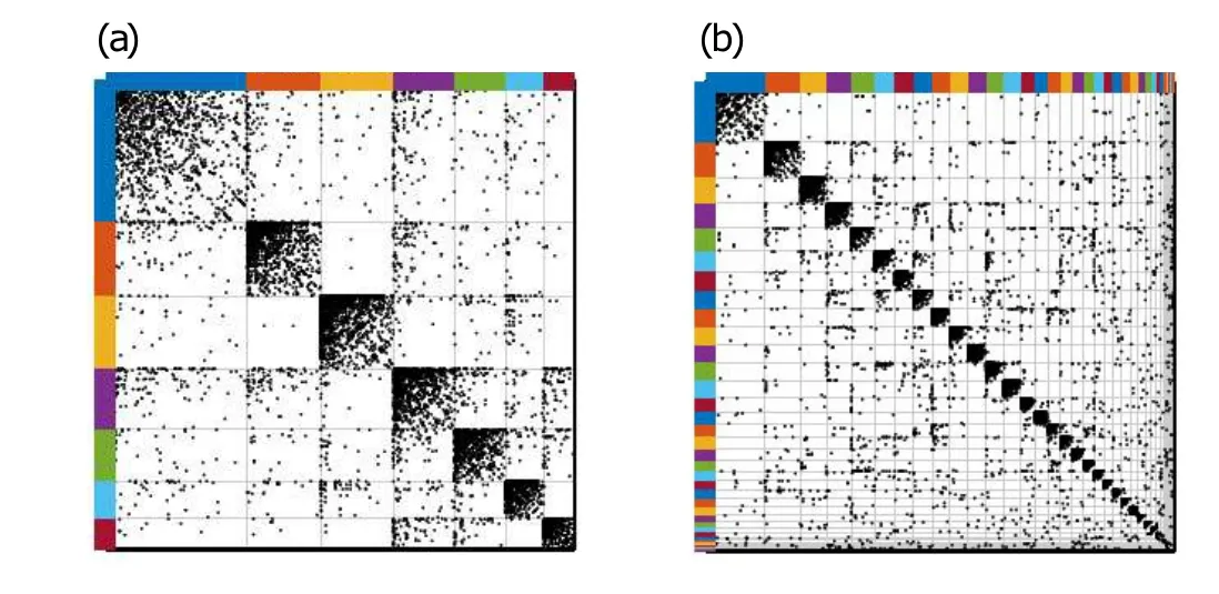
Fig. 10. (a) Ground-truth communities of “Cora”; (b) clustering results of“Cora”by PYP-IP.
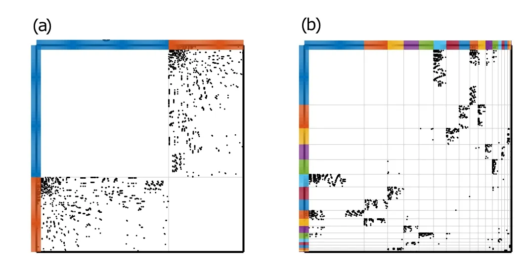
Fig.11. (a)Ground-truth communities of“Mus-ske”;(b)clustering results of“Mus-ske”by PYP-IP.
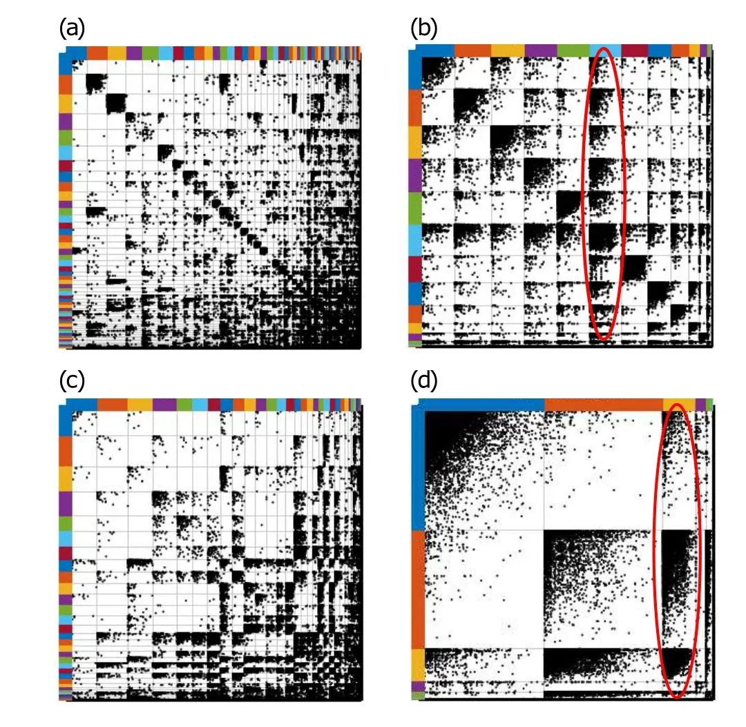
Fig.12. Blocks detected by DCSBM compared with PYP-IP:the communities detected by DCSBM result in denser links in a block or between blocks,which cause the interaction patterns to fade away. (a) Clustering results of “Eu-core” by DCSBM; (b) clustering results of “Eu-core” by PYP-IP;(c) clustering results of “Poli blog” by DCSBM; (d) clustering results of“Poli blog”by PYP-IP.
5. Conclusions and future work
In this paper,we propose the model,PYP-IP,for detecting communities based on vertices’latent interaction-patterns,and it uses the Bayesian nonparametric, i.e., Pitman–Yor process as a prior for vertex partitions.We prove that PYP-IP can characterize and detect various community structures including assortative community structure, bipartite community structure and disassortative community structure without knowing the type of community structures beforehand. The number and sizes of communities can be estimated automatically through a collapsed Gibbs sampling approach.Then,we evaluate PYPIP on the networks with different community structures. The experiment results show PYP-IP is competent to explore various community structures. Finally, the visualizations of the adjacency matrix with grouped vertices show some hidden interaction patterns,and can also be revealed by PYP-IP,which will offer extra information for network analysis.
The joint merge-split moves of a group (Ref. [32]) may improve the efficiency of our MCMC algorithm, but the improvement may be a little bit.[55]CRMSBM[34]based on complete random measure owns more theoretical mathematicbackground,i.e.,random measure,which is an advanced tool that can analyze big data and random events, so it has many merits we should learn. More nonparametric priors can be applied in the model to make it more flexible for sparse networks.The hierarchical extension also can be considered to explore more complex structure in the networks.
猜你喜歡
Chinese Physics B(2022年3期)2022-03-12 07:44:46
美與時代·城市版(2021年9期)2021-10-30 14:50:55
大眾文藝(2021年16期)2021-09-11 09:05:06
知音海外版(下半月)(2020年6期)2020-07-16 18:18:41
電影(2019年6期)2019-09-02 01:42:28
中華建設(shè)(2019年2期)2019-08-01 05:57:48
閩商文化研究(2019年2期)2019-05-21 07:25:58
Journal of Oceanology and Limnology(2018年3期)2018-07-11 01:58:30
神經(jīng)損傷與功能重建(2018年1期)2018-01-31 20:02:28
Transactions of Nanjing University of Aeronautics and Astronautics(2015年5期)2015-02-09 06:08:58

- Chinese Physics B的其它文章
- Modeling the dynamics of firms’technological impact?
- Sensitivity to external optical feedback of circular-side hexagonal resonator microcavity laser?
- Controlling chaos and supressing chimeras in a fractional-order discrete phase-locked loop using impulse control?
- Proton loss of inner radiation belt during geomagnetic storm of 2018 based on CSES satellite observation?
- Embedding any desired number of coexisting attractors in memristive system?
- Thermal and mechanical properties and micro-mechanism of SiO2/epoxy nanodielectrics?