Adaptive ANCF method and its application in planar flexible cables

Yue Zhang·Cheng Wei·Yang Zhao·Chunlin Tan·Yongjian Liu

1 Introduction

Since proposed,ANCF has become the hot topic of multibody system dynamics.Most of the papers focus on element technology,including the cable/beam elements[5–10],plate/shell elements[11–14],and solid elements[15].These papers at tempted various approaches to modify and optimize ANCF elements to enhance the kinematical and dynamical performance.With the rapid development of element technology,the ANCF method has become widely applied in many flexible multi-body systems,such as pulley-belt/cable systems[16–19],railway catenaries[20,21],vehicle tires[22,23],and liquids[24],etc.Asa discrete modeling method,the ANCF will bring in discretization errors for flexible dynamic systems.The dynamical environment is usually very complex,the probably existing alternating and concentrated loads will cause large and complex deformations,especially for flexible bodies with low stiffness.Therefore,it is difficult to definitely determine how to generate mesh for various dynamical systems to ensure the computational accuracy.In general,a satisfactory accuracy can be obtained if the mesh is dense enough,but this will result in a poor computational efficiency.So,it will be a significant and challenging work to ensure the accuracy,and meanwhile enhance the computation efficiency.

The accuracy of flexible dynamics is not only related to the mesh density,but also related to the motion state of flexible bodies.The discretization error tends to be larger when the flexible bodies undergo large and complex deformations.In many situations,the large deformations only exist in some small local domains,and these local domains are alterable and cannot be determined beforehand.So the whole domain of the flexible body needs to be densely meshed just to ensure the accuracy of these local domains,which results in unnecessary loss of computational efficiency.

The above problem is common in flexible multi-body dynamics,and it is particularly serious for large-scale and low-stiffness flexible multi-body systems.Similar problems also exist in the statics analysis when the finite element method(FEM)is used.The FEM is capable of producing accurate approximate solutions for the statics problems,but there are still errors produced by the finite element model when the interpolation functions are incapable of representing the complexity of the exact solution on the domain of the individual elements[25].Usually the finite element model is uniformly meshed,and dense meshes are needed to meet the accuracy demand in the whole domain,which results in a poor computational efficiency.Therefore,the adaptive finite element method(AFEM)was developed in the early 1980s to improve the models with adaptive refinement[26–29].In AFEM,the error estimation and mesh refinement are the core techniques.In terms of error estimation,Babuska and Rheinboldt[28,30]proposed the residual error estimate method,and an efficiency indicator was given to evaluate the reliability of error estimate method.In addition,Zienkiewicz and Zhu[31–33]proposed a posterior error estimator(Z/Z error estimator),they estimated the discretization errors by the stress smoothing technique.Meanwhile,Ainosworth et al.[34]proved the effectiveness of the Z/Z error estimator,and then Choudhardy and Grosse[35]further promoted this method.The mesh refinement strategies mainly include h-refinement,p-refinement and r-relocation.In the h-refinement[36],the elements will be divided into lots of small elements,if the elements have a significant amount of error.The h-refinement is simple and easy to implement,so it is most widely used in AFEM.P-refinement[37]increases the order of interpolation functions without changing the mesh,it is difficult to ensure the convergence of the refinement process,because it highly depends on the initial mesh.R-relocation[38,39]decreases the discretization error by redistributing the nodes,the number of elements and the order of the interpolation functions is unchangable during the process of refinement.In addition,the mesh can also be refined by using the combination of these strategies to cover the shortage of a single strategy[40–42].

Similarly,an adaptive absolute nodal coordinate formation(AANCF)is presented to improve the accuracy and efficiency of dynamic computation.In AFEM,the mesh is usually densified iteratively(h-refinement)to acquire a satisfied accuracy,while in AANCF,the mesh should also be sparsified to improve the efficiency.Therefore,the strategy of element merging is proposed in the AANCF cable model.In addition,the adaptive optimizations exist in the dynamic computation process,the mesh will be updated,and the dimension of dynamic equation will not be constant any more,so the continuity of dynamic status is another key problem to be considered,while this is not a problem in AFEM.In this paper,the continuity of AANCF cable is analyzed to seek the key factors that affect the continuity,and based on the continuity analysis,a continuity-optimized AANCF model is given to further improve the AANCF model.In general,the AANCF will be more complicated and involves more issues compared with AFEM.

2 Movement features of flexible bodies

The movements of flexible bodies are different in various situations,but there are still some common features,especially for the low-stiffness flexible bodies,which can be summarized as follows:

(1)Large-scale motion accompanying complex deformations:influenced by a complex dynamical environment,such as the alternating load and concentrating load,etc.,the flexible body tends to form large and complex deformations during the large-scale motion.

(2)Space-varying deformations:the deformations of flexible body are space-varying,the magnitude and complexity of deformations in various domains are different,and in many situations,the large and complex deformations only exist in some small local domains.

(3)Time-varying deformations:the deformations of flexible body are time-varying,for instance,a previous small deformed domain may undergo large deformations after a period of time,and vice versa.

(4)Unpredictability of deformations:as the deformations of a flexible body are space-varying and time-varying,one cannot know when,where,and how the deformations will occur,so the deformations are unpredictable.

3 Conventional and adaptive ANCF method

The flexible cable in Fig.1 is taken as an example to illustrate the two dynamic simulation methods:the conventional ANCF and the adaptive ANCF.

The flexible cable,with one end fixed,falls from a horizontal position under gravity.At the beginning(t=0),the flexible cable has no deformation,as time goes on,the deformations occur with the movement of flexible cable.According to the movement features analyzed above,one cannot predict when,where,and how the deformations will occur to the flexible cable.For example,the deformations may be not very large att1,while when the time comes tot2,large deformations may occur near the fixed end of the flexible cable.

Conventional ANCFIn conventional ANCF,the model is pre-meshed,the number,distribution and type of elements are unchangeable during the simulation.If the model is sparsely meshed(Fig.1a),the elements cannot well capture the complexity of the exact solutions when the large and complex deformations occur in some domains(e.g.,the root domain att=xt2).Therefore,although the sparse-mesh model has satisfactory accuracy when the deformations are small and simple(e.g.,att=0 andt=t1),it cannot ensure the accuracy during the whole simulation.Due to the unpredictability of deformations,the model is usually densely meshed to ensure the accuracy during the whole simulation(Fig.1b).As the large and complex deformations may only occur in some small local domains and last for a short period of time,the dense-mesh model will result in a great efficiency loss.

Adaptive ANCFThe specific movement features of flexible bodies make it difficult to ensure the accuracy with the unchanged mesh during the whole simulation.So the mesh can be adaptively modified with the movement of flexible bodies.At the beginning,the model can be still sparsely meshed,while with the increase of the magnitude and complexity of deformations,the mesh is densified to obtain a satisfactory accuracy(Fig.1c).The adaptive ANCF method can ensure the accuracy during the whole simulation,and meanwhile avoid the unnecessary loss of efficiency.

4 Computation strategy of AANCF

The dynamic equation of a flexible body based on continuum mechanics is a partial differential equation,in which the time and material coordinates are the independent variables.In most situations,the analytical solution is unavailable,so the discretization method is applied,and it brings discretization errors to dynamical systems.According to the movement features of flexible bodies discussed above,there should be an optimal mesh at each moment to meet the accuracy demand with minimum degrees of freedom.The AANCF method is just an attempt to optimize the mesh during dynamic computation.

As can be seen in Fig.2,the adaptive computation is started by model initialization based on the initial input data,including constraint and loading conditions,geometry and material properties,element sizes in initial mesh and initial positions and velocities.In the initialization phase,the mesh is generated and the dynamic equation is formed.Generally,the dynamic equation is a differential algebra equation(DAE)with the following form:

Fig.1 Dynamic simulation of flexible cable with different methods.a Sparse mesh.b Dense mesh.c Adaptive mesh

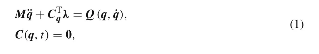
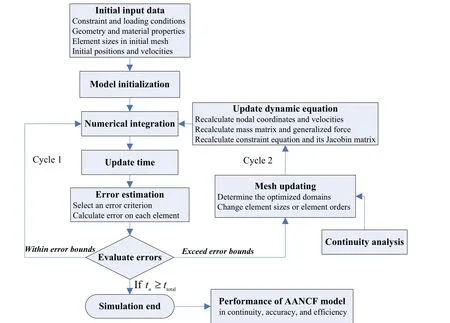
Fig.2 Adaptive computation strategy

whereQ(q,˙q)is the generalized force,and it consists of external and elastic forces.

In order to get the dynamic responses of the flexible system,the DAE should be solved by numerical integration.After this,the discretization error is estimated to provide error criterion for the adaptive computation.If the errors in some domains exceed the error bounds which are set in advance,the meshes in these domains will be regenerated through changing element sizes or element orders(cycle 2).After the modification of the mesh,the dimensions of the dynamic equation are changed,the nodal coordinates and velocities,mass matrix,generalized force,constraint equation,and its Jacobin matrix should be recalculated to update the dynamic equation.If the errors are within the error bounds,the simulation circle 1 will be entered without element updating.

It is important to note that the modification of the mesh may cause sudden changes in dynamic status.The discontinuity will reduce the accuracy to some extent,and the corresponding errors will be accumulated in the subsequent simulation.Moreover,the jumps of dynamic variables may affect the calculation stability and cause greater distortion.So,in order to restrict the possible jumps of dynamic variables,the continuity should be analyzed before the optimization strategy is determined.

The AANCF is an adaptive dynamic approach in temporal and spatial domains,where the error estimation and mesh updating are the core techniques.In addition,after the adaptive computation,it is necessary and important to evaluate the performance of the AANCF model for further study and improvement.So,the important issues such as error estimation,mesh updating and performance of the AANCF model are further discussed in the next section.

5 Important issues of AANCF

5.1 Error estimation

The discretization error is the error between the ANCF solution and the exact solution of the governing partial differential equation.It belongs to modeling error and will make the solu-tion lose its significance if the model is not meshed properly.The object of error estimation is to provide a criterion for the adaptive optimization of mesh.In the following,three error estimation methods are provided,where some ideas of error estimation of AFEM are used for reference.

Residual error methodIn most situations,the analytical solution of the governing partial differential equation is in accessible,which means the exact solution of flexile dynamics cannot be obtained directly.If we substitute the solution of ANCF into the governing equation,the equation will not be balanced anymore,and the more accurate the ANCF solution is,the smaller the residual error will be.So the residual error of the governing equation can be used to evaluate the discretization error of ANCF.But for most flexible multibody systems,the governing partial differential equation is difficult to obtain,so the residual error method is not very suitable for practical engineering problems.

Approximate solution methodAlthough the exact solution of flexible dynamics cannot be obtained directly,the discretization error still can be estimated based on the approximation of an exact solution.In general,the ANCF element can ensure the first order continuity,but for variables with second derivatives,such as the curvature and bending moment,there exist jumps between the elements.Through interpolating the discontinuous strain or stress,a smooth solution of strain or stress,which is closer to the exact solution,can be obtained.Thus,the smooth solution can be used to estimate the discretization error instead of the exact solution.This method is similar with the Z/Z error estimate method in AFEM[31],but for the dynamic problems in AANCF,the error of change rate of strain or stress should also be estimated to meet higher accuracy demands.The approximate solution method is an intuitive idea,and the mathematical basis is not enough relative to the residual error method.But the governing equation is not needed in this method,the error can be estimated only with the ANCF solution,so this method is more convenient for the adaptive computation.

Indirect estimation methodIn the approximate solution method,constructing the smooth solution after each integration step will cost some time and cause an efficiency loss.In AFEM,the inter element jump in the strain or stress can quantify the discretization error and serve as the error criterion for adaptive optimization[25,43].Similarly,one or several simple variables like the inter element jump can also serve as the error criterion in AANCF to simplify the error estimation process.Besides,there can be specific error criteria for specific elements and simulation conditions.For example,for the plate and beam elements with a membrane locking problem,the larger the bending deformation is,the more serious the element distortion will be.Therefore,the magnitude of bending deformation can serve as the error criterion for the adaptive computation.Although these indirect estimation methods have no strict theoretical basis,they may be more practical and effective in some engineering problems.

5.2 Mesh updating

In AFEM,the mesh can be optimized by reducing the size of elements(h-refinement),increasing the order of interpolation functions(p-refinement),relocating the element nodes (r-relocation)orusing the combination of them,and the mesh should be constantly modified through iterative calculation until the demanded accuracy is achieved.But for AANCF,the mesh is modified in the simulation process,so the continuity of dynamic status should be considered.As it is difficult for ther-relocation technique to ensure the continuity of dynamic status,this technique will not be used in AANCF.The mesh can be optimized by changing the element sizes or polynomial orders.For instance,when the errors in some domains exceed the upper error bound,the elements in these domains will be divided or the polynomial orders will be enhanced to reduce the errors,conversely,the elements will be merged or the polynomial orders will be reduced to enhance the efficiency.The mesh updating process does not involve iterative calculation,and generally it only occupies a small number of steps in the whole simulation.

5.3 Performance of AANCF model

ContinuityThe continuity of simulation results is an important indicator to reflect the performance of AANCF model.In the spatial domain,the higher-order strains are discontinuous(e.g.,the curvature of first-order continuous elements),and generally the continuity of strains can be improved by the adaptive computation.In the temporal domain,dynamic variableslike displacement,velocity,acceleration,strain and energy,etc.,may have jumps when the mesh is modified,so the continuity of these variables should also be evaluated.AccuracyThe purpose of adaptive computation is to improve the accuracy and efficiency of flexible dynamics.The theory of the finite element method indicates that when the mesh is constantly densified,the FEM solution will convergence to the exact solution of the governing equation.For most flexible dynamics systems without analytical solutions,the ANCF model with denser meshes can serve as the standard to investigate the accuracy of the AANCF model.To better reflect the performance of the AANCF model,the accuracy should be overall analyzed both in the temporal domain(e.g.,analyzing the changes of displacement,velocity,and energy,etc.)and the spatial domain(e.g.,analyzing the configuration,strain,and stress,etc.,in different areas).EfficiencyThe computational efficiency is influenced by many factors,such as integration step,number of iterations,and dimension of equation,etc.,where the dimension of the equation depends on the model itself,while the integration step and the number of iterations are influenced by both the dynamic model and the numerical algorithm.Thus,by analyzing these factors and comparing the AANCF model with the conventional ANCF model under the same level of accuracy,the efficiency improvement of AANCF model can be evaluated.

6 Differences between AANCF and AFEM

In AANCF,some ideas of AFEM are used for reference,but there are still some differences between AANCF and AFEM:

(1)The AFEM focuses on the statics problems,the mesh is optimized iteratively after the statics calculation until the errors fall below the permissible value.The AANCF focuses on the dynamic problems(especially for large deformation problems),the mesh is optimized during the calculation.

(2)The AFEM is an adaptive computation method in the spatial domain,while the AANCF is an adaptive computation method both in the temporal and spatial domains.Therefore,the calculation errors will be accumulated in the subsequent simulation,which means the errors should be more strictly controlled.

(3)In AANCF,the dynamic status may be discontinuous when the mesh is modified during the calculation.The discontinuity has a bad influence on the stability and accuracy ofthe calculation,so the continuity of dynamic status should be analyzed before the optimization strategy is determined.However,there is no such problem in AFEM.

7 Theoretical model of AANCF cable

7.1 ANCF cable element

In this part,the cable element model is established based on Ref.[7],and the element-related parameters are seen in Fig.3.

The generalized coordinates which consist of the position vector and the position vector gradient atx=0 andx=Lcan be written as

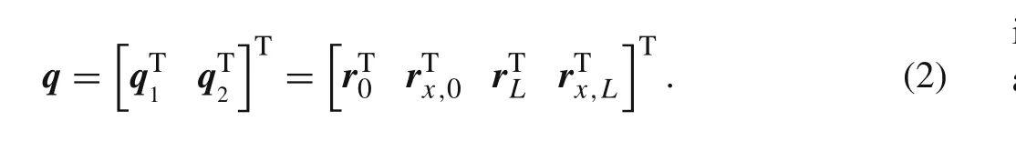
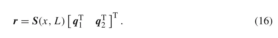
The displacement field of a cable is expressed as

Fig.3 Diagram of cable element

whereS(x,L)is the shape function and is given by

As the shape function is time-independent,the velocity vector of an arbitrary point on the cable centerline is˙r=S˙q.Suppose the density and cross-section area areρandA,then the kinetic energy of cable element can be written as

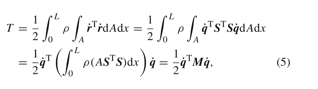
whereMis the mass matrix,and it is expressed as

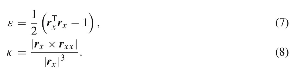
The axial and bending deformations are taken into account in this cable element,and the deformations are described by axial strainεand curvatureκas

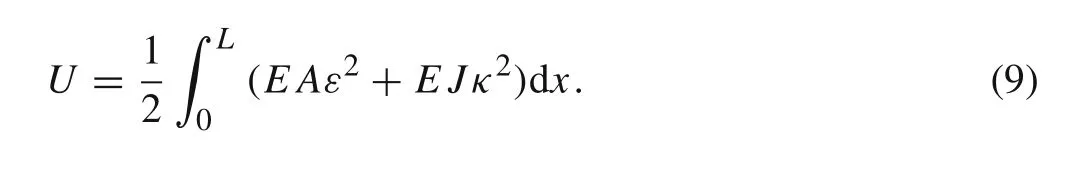
According to the Euler–Bernoulli beam formulation,the strain energy of a cable element is

Considering the viscoelasticity of material,the generalized force of cable element can be written as

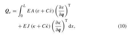
whereEandJare the elastic modulus and moment of inertia of the cable cross section,Cis the damping coefficient.

7.2 Adaptive computation based on the bending angle of an element

As mentioned earlier,the error criterion for element updating is crucial to the AANCF cable model.Due to the kinematics description of cubic Hermite interpolation,there exists curve induced distortion(CID)[44]in the ANCF cable:changes in the state of curvature cause changes in the distribution of points along the curve.Therefore,the bending deformation of the cable will lead to nonuniform and fictitious axial deformation,causing the element to be overly stiff and inaccurate.For a certain element,the larger the bending deformation is,the more serious is the CID effect.So the bending angle of an element will serve as the error criterion for element updating.

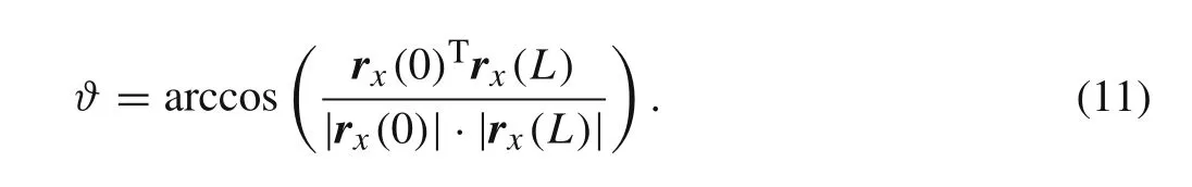
The bending angle of an element?is defined as the included angle between two tangent lines at the ends of an element

7.2.1 Dividing elements

In order to improve simulation accuracy,the cable elements can be automatically divided if the bending angles of some elements exceed the upper bound?max.For example,if

the elementiwill be divided into two new elements by adding a new node in the element center,as can be seen in Fig.4,whereiandjare the symbols of element and node,respectively.

After being divided,the original element turns into two new elements with half of the original length.So the dimension of dynamic equation,mass matrix and generalized force will be changed,in addition,the generalized coordinates and generalized velocities need to be updated.

The generalized coordinates of the new added node

Fig.4 Element division.a Before dividing.b After dividing

The generalized velocities of the new added node

7.2.2 Merging elements

In order to improve the simulation efficiency and meanwhile ensure the accuracy,the adjacent elements can be merged if the bending deformations are not very large.For example,if the overall bending angle of adjacent elements?i,i+1is smaller than the lower bound?min,the adjacent elements will be merged through deleting the common node.

It should be noted that the bending directions of elementiand elementi+1 might be the same or opposite,as can be seen in Fig.5.If the elements are bending in the same direction,then?i,i+1=|?i+?i+1|,which ensures?i＜?min,?i+1＜?min;if the elements are bending in the opposite direction,then?i,i+1=|?i??i+1|,on this occasion,?ior?i+1might be very large and?i＜?min,?i+1＜?mincannot be ensured any more.So,the adjacent elements can be merged only when the bending directions are the same.

Although the element error would be very small when the cable undergoes small deformations,the error still cannot be ignored,be cause it will be accumulated overtime.Therefore,the length of merged element should not be too large.An upper boundLmaxis set to restrict the element length,that isL i+L i+1≤Lmax.

According to the above analysis,the adjacent elementsiandi+1 can be merged only if the following conditions are satisfied

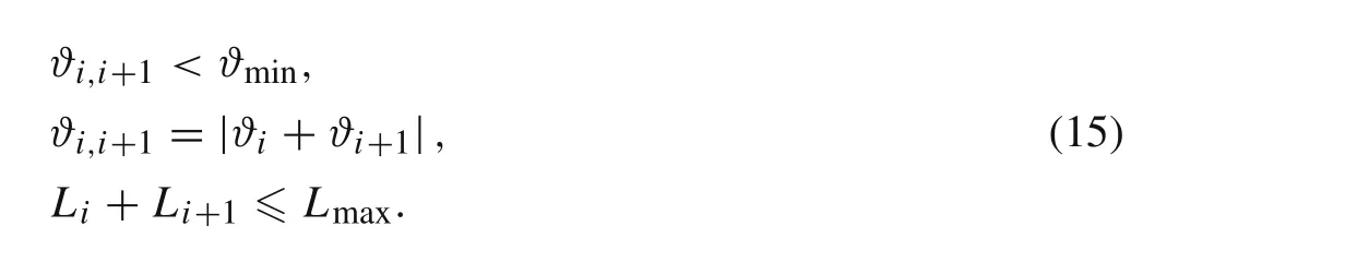
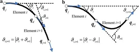
Fig.5 Bending deformations of adjacent elements.a Bending in the same direction.b Bending in the opposite direction

7.3 Continuity analysis

In the adaptive computation process,the number and size of elements will be changed.If the dynamic state jumps obviously after element division or merging,the computational accuracy and stability will be adversely affected.So the continuity of dynamical variables like displacement,velocity,strain,and energy will be discussed in this section.For the convenience of theoretical derivation,the symbolsq j,q j+1in Figs.4 and 5 are substituted byq1,q2.

7.3.1 Dividing elements

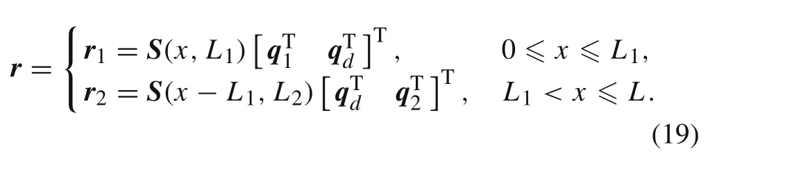
The original displacement field before element division is

After the element is divided,the displacement field turns out to be

Spread Eqs.(16)and(17),the displacement fields before and after element division can be written as

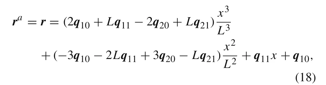
whereq10=r0,q11=r x,0,q20=r L,q21=r x,L.According to the above equation,the displacement fields before and after element division are completely equivalent,so the displacement is continuous.

Moreover,equations˙r a=˙r,r ax=r x,andr axx=r xxcan be obtained by Eq.(18).As the axial and bending strains only depend onr xandr xx(Eqs.(7)and(8)),and the energy is only related to the velocity and strain(Eqs.(5)and(9)),the velocity,strain and energy are also continuous.

7.3.2 Merging elements

Suppose the lengths of adjacent elements to be merged are respectivelyL1andL2,and the length of merged element isL=L1+L2.The displacement field before element merging can be written as

After the elements are merged,the displacement field turns out to be

SupposeL1=ζL,L2=(1?ζ)L,0＜ ζ＜1,then the difference of displacement fields can be written as

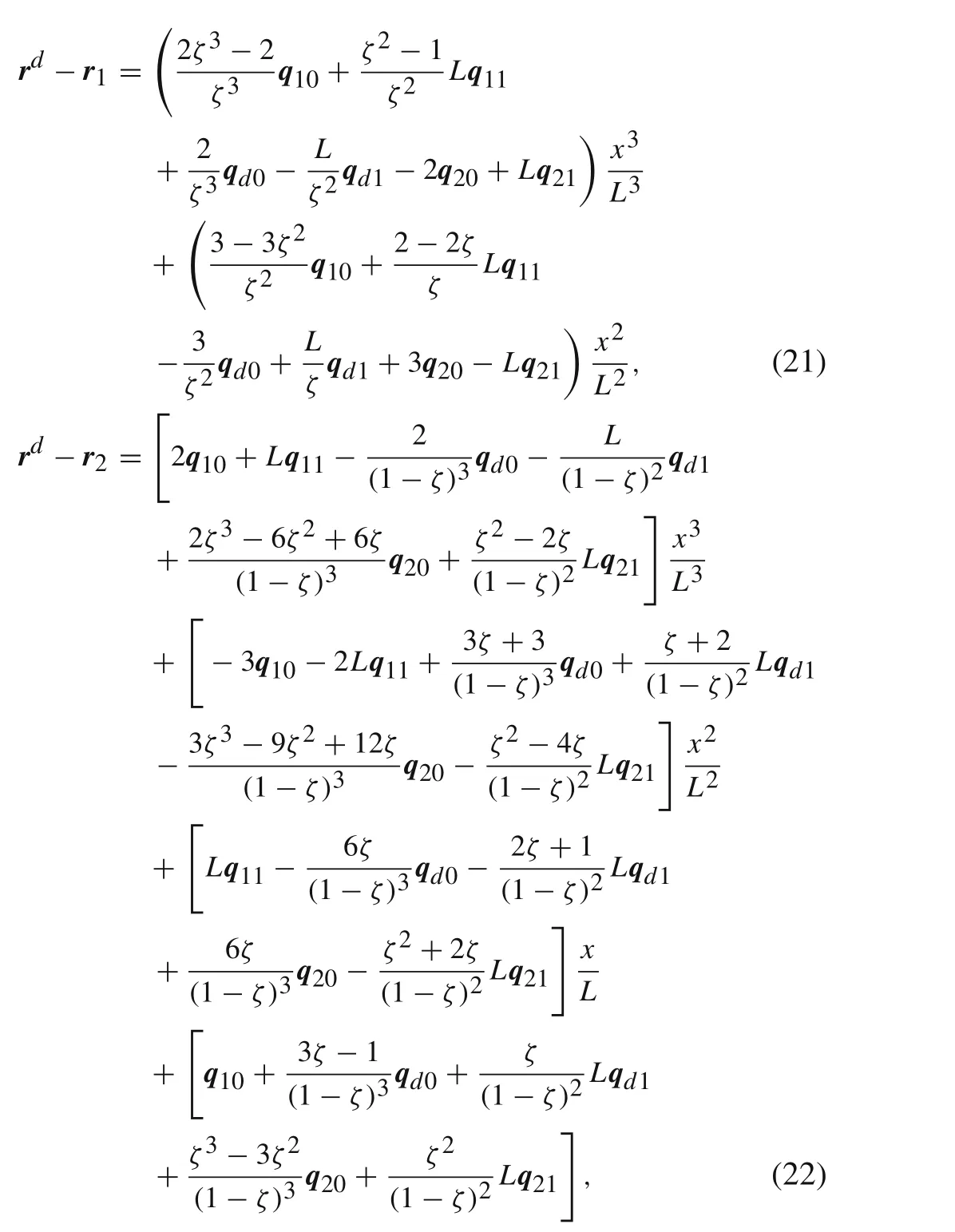
whereq d0=r L1andq d1=r x,L1are,respectively,the displacement and gradient of the deleted node.After the elements are merged,the displacement and gradient of the deleted node turn out to be

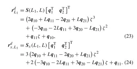
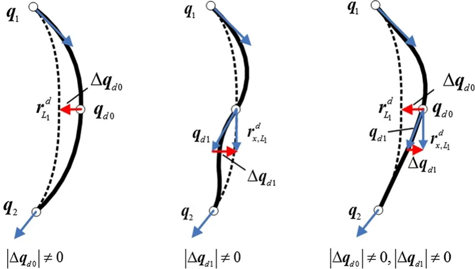
Fig.6 Influence of Δq d0 and Δq d1 on the displacement field

Substitute Eqs.(23)and(24)into Eqs.(21)and(22),the difference of displacement fields can be simplified as

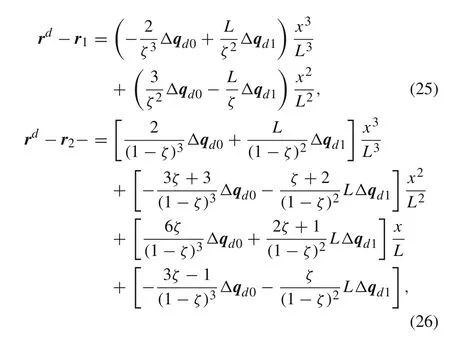
whereΔq d0=r dL1?q d0, Δq d1=r dx,L1?q d1,which represent the jump values of the displacement and gradient of deleted node,respectively.For certain adjacent elements,the difference of displacement fields is only related toΔq d0andΔq d1.The influence ofΔq d0andΔq d1on the displacement field can be illustrated by Fig.,where the solid and dashed lines are,respectively,the cable con figurations before and after element merging.IfΔq d0=0,Δq d1=0,the displacement fields before and after element merging will be identical.Otherwise,the displacement will not be continuous any more,and the largerworse the continuity of displacement will be.According to Sect.7.3.1,the continuity of velocity,strain and energy is closely related to the continuity of the displacement field,so the continuity of velocity,strain and energy also depends on the values ofΔq d0andΔq d1.

8 Numerical study of the AANCF cable

8.1 Simulation of the AANCF cable

The flexible cable in Fig.1 is simulated in this section,where the length and diameter of the flexible cable are,respectively,3 and 0.01 m,the elastic modulus and damping coefficient are,respectively,2×109Pa and 0.1,the upper and lower bounds of bending angle are,respectively,set as 0.6 and 0.25 rad,the maximum length of the element is set as 0.9 m.The Hilber–Hughes–Taylor(HHT)algorithm[45]is used to solve the dynamic equation.

Figures 7 and 8 display the simulation results of the AANCF cable,where Fig.7 shows the configuration of the flexible cable at different times,and Fig.shows the variation of the number of elements.The flexible cable is divided into six elements of equal length at the beginning,as time goes on,the number of elements starts to change with the division and merging of elements.Before 1.8 s,the number of elements shows an increasing trend,only at 0.54 and 1.03 s,the number of elements decreased with the merging of elements,where the merged elements are circled in Fig.7a.Most of the new added elements are concentrated in the root domain(see Fig.7),because the flexible cable near the fixed end undergoes a larger bending deformation.The number of elements in the root domain increases from 1 to 6,leading to a dense element distribution at the fixed end:the smallest element length reaches 0.0625 m,only 1/8 of the original length.After1.8 s,the bending deformations of elements start to decrease and the elements are merged.It is easily seen that the elements are gradually merged in the root domain with the deletion of nodes,in addition,the elements are also merged in the other domains,and the largest element length reaches 0.75 m,as can be seen in Fig.7b.Although the number of elements has a slight increase from about 2.3 to 2.5 s,it still decreases to six ultimately.But at this moment,the distribution of elements is obviously different from the initial state.According to the above analysis,it is obvious that AANCF is an adaptive computation method in temporal and spatial domains.

To analyze the accuracy of the AANCF cable compared with the conventional ANCF model,the convergence property of the ANCF cable should be discussed first.Figure 9 shows the displacement curves of an endpoint with different numbers of elements(6,12,24,36).According to the if gure,there is a relatively large difference between the displacement curves of the 6-element model and the 12-element model,while with the increase of the number of elements,the displacement curves are getting closer and closer,the relative error between the 24-element model and the 36-element model is smaller than 0.3%.Therefore,the36-element model will be used to evaluate the accuracy of the AANCF cable in the following.

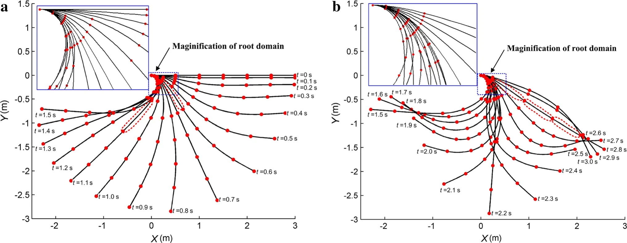
Fig.7 Configuration of flexible cable at different times.a 0–1.5 s.b 1.5–3 s

Fig.8 Variation of the number of elements

8.1.1 Accuracy and efficiency

In order to analyze the accuracy of the AANCF cable in temporal and spatial domains,the displacement,velocity,and configuration of the flexible cable are presented and discussed in this section.

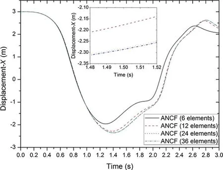
Fig.9 Displacement of endpoint of conventional ANCF cable

The movement of the endpoint of the conventional ANCF cable and AANCF cable are compared in Figs.10 and 11,where the 36-element model is used to evaluate the accuracy of different models.The displacement and velocity curves of the three models are almost coincident with each other in the initial stage.While,with the increase of element deformation and decline of element accuracy,the displacement and velocity curves of 6-element model gradually separate from the curves of 36-element model from 0.6 s inxdirection and 0.7 s inydirection,and as time goes on,the errors are getting larger and larger.Different from the 6-element model,the curves of the AANCF model are much closer to those of 36-element model,which means the AANCF model has a relatively high accuracy.

To analyze the accuracy of the cable in the spatial domain,the configuration of different cable models at 0.5,1.0,1.5 s are compared in Fig.12.The position curves of the 6-element model have big deviations from those of the 36-element model,and the deviations mainly exist in the root domain.And it is obvious that the bending deformations of the 6-element model are smaller than those of the 36-element model,especially at 1.0 and 1.5 s.While for the AANCF model,the position curves are very close to those of the 36-element model.

The reason for these phenomena can be explained as follows:the fixed end of the bears a concentrated load,and the large bending deformation in this domain makes the CID effect more significant when large-sized elements are applied in the 6-element model.While for the AANCF model,the elements are divided into smaller ones with the increase of deformation.For example,the number of elements in the root domain(0–0.5 m)are respectively 2,4,6 at time 0.5,1.0,1.5 s.Thus the elements can still remain at small bending angles and keep a high accuracy even though the cable undergoes larger deformation in the root domain.In addition,there is a little error in the small-deformed domain(0.5–3 m)because the elements are still sparsely distributed,even so,the error is much lower than that of the 6-element model.

The accuracies of some main dynamic variables were discussed in the above analysis,and it can be seen that the accuracy of the flexible cable is obviously improved by the AANCF method.In spite of this,it would be unworthy to introduce the AANCF method if the efficiency is greatly reduced,because improving the computational efficiency is a main purpose of using this method.

Compared with the conventional ANCF cable,the efficiency improved by AANCF cable is mainly reflected in the number of elements when the same numerical algorithm is applied.As the number of elements is not constant(as seen in Fig.8),the average number of elements during the simulation is applied to evaluate the efficiency.According to Fig.8,the average number of elements is 9.3,which can be obtained through dividing the shadow area by simulation time.It can be seen that the AANCF model has greatly improved the accuracy with only a slight decrease of efficiency(6-element model),and compared with the 36-element model,the AANCF model possesses a much higher efficiency.

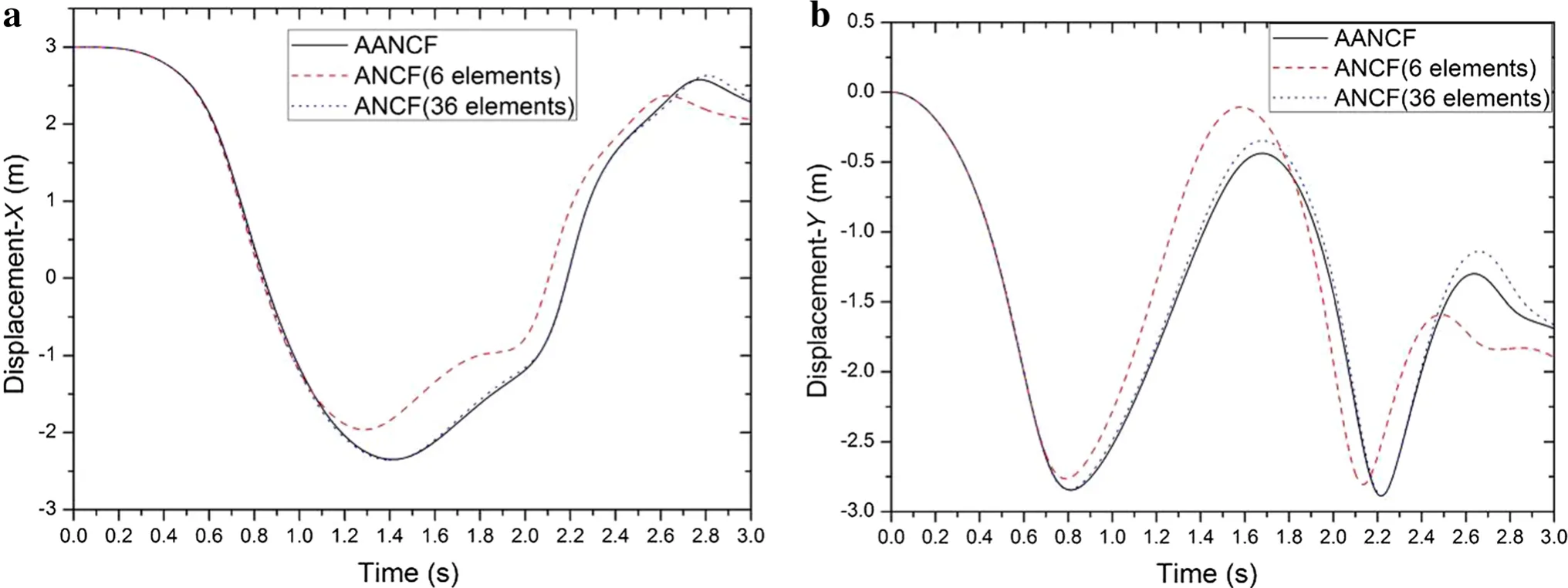
Fig.10 Displacement of endpoint.a Displacement in x direction.b Displacement in y direction

Fig.11 Velocity of endpoint.a Velocity in x direction.b Velocity in y direction

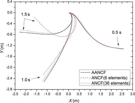
Fig.12 Configuration of different models

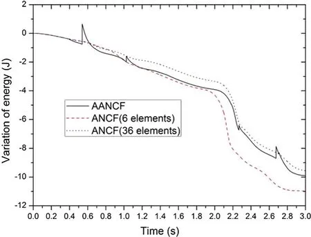
Fig.13 Variation of system energy

8.1.2 Continuity

According to the analysis in Sect.7.3,the dynamic state is probably discontinuous when the adjacent elements are merged.The variation of system energy is given in Fig.13 to analyze the continuity of the AANCF model in the temporal domain.According to Fig.13,there exists some large sudden changes in the energy curve of the AANCF model,respectively,at 0.54,1.03,2.26,2.67 s.It is just in these moments that the elements are merged,and thus caused the energy jumps.Even so,compared with the 6-element model,the energy curve of the AANCF model is closer to the one of the 36-element model.

Figure 14 shows the curvatures of different models at 1.5 s.It can be seen that the curvature of the AANCF model is much more accurate than that of the 6-element model.Besides,the curvatures are not continuous,there exist jump values at the nodes.The jump values of AANCF model are smaller than those of 6-element model,especially in the root domain.So the AANCF model has a better curvature continuity compared with the conventional 6-element model.

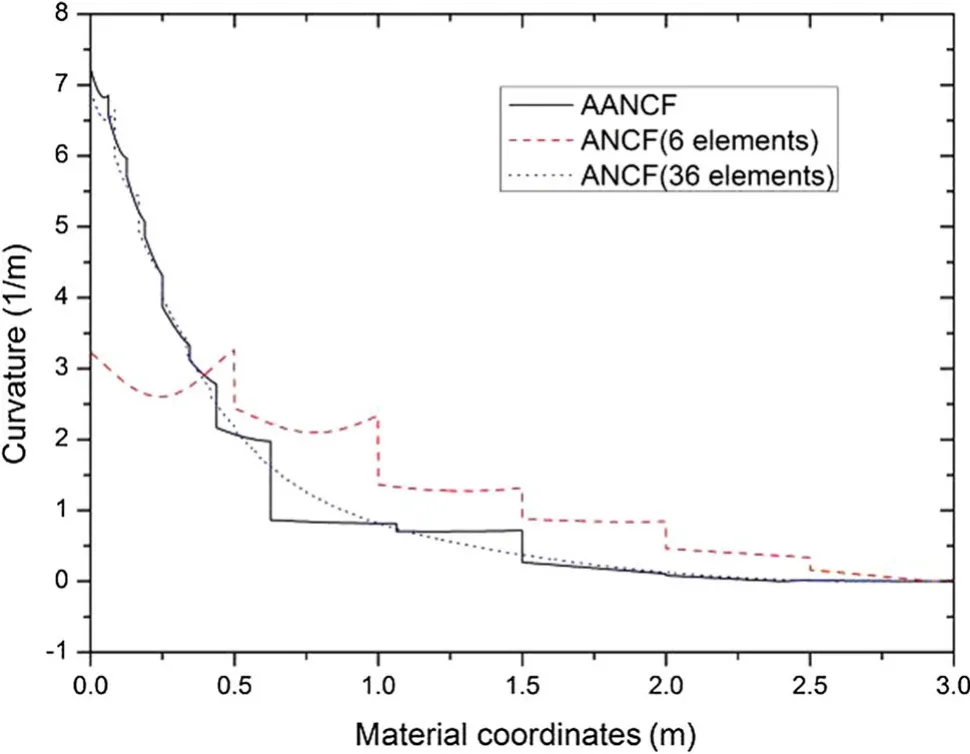
Fig.14 Curvatures of different models at 1.5 s

8.2 Continuity optimization of AANCF cable

The simulation results of the continuity-optimized AANCF model are presented and compared with other models in Fig.15.It can be seen from Fig.15a that the jumps of energy in the AANCF model do not exist in the continuity-optimized AANCF model any more,which means the continuity of energy is obviously improved.According to Fig.15b,the variation trends of the number of elements before and after continuity optimization are quite similar,but for the continuity-optimized AANCF model,the elements are not merged at0.54 and 1.03 s,and the moments of element merging after 2.1 s have a little difference with those of AANCF model.This means the continuity-optimized AANCF model selected a more appropriate time to merge elements,which explains why the continuity of system energy is improved.According to Fig.15c,d,after the continuity is optimized,the accuracy of displacement has a further improvement on the basis of the AANCF model.So,compared with the AANCF model,the continuity-optimized AANCF model has better performances in both accuracy and continuity.

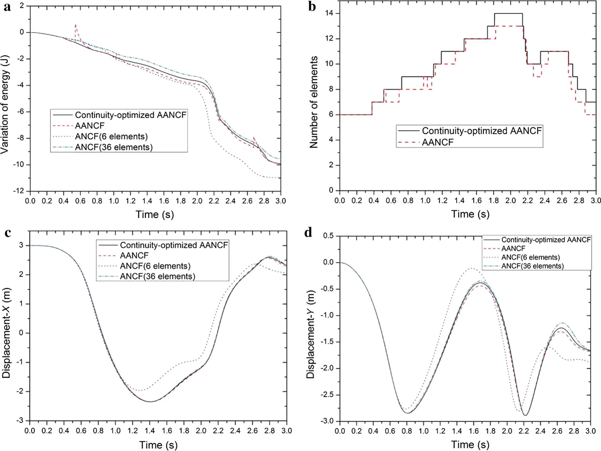
Fig.15 Results of the continuity-optimized AANCF cable.a System energy.b Number of elements.c Displacement of endpoint in x direction.d Displacement of endpoint in y direction

9 Conclusions

In order to improve the accuracy and efficiency of flexible dynamics,an adaptive ANCF method is proposed in this paper.In this method,the mesh can be adaptively modified during dynamic computation to ensure the accuracy in both temporal and spatial domains.

(1)The computation strategy of AANCF is provided based on the movement features of flexible bodies.Then,the important issues such as error estimation,adaptive optimization,the performance of the AANCF model are discussed in detail,and the differences between AANCF and AFEM are summarized.

(2)The theoretical model of the AANCF cable is presented,in which the strategies of dividing and merging elements are discussed.The criterion for element division is the bending angle of the individual element,while the criterion for element merging is more complicated,expect for the overall bending angle of adjacent elements,the bending directions of adjacent elements and the length of merged element should also be considered.

(3)The continuity is theoretically analyzed,it is found that the dynamic state is probably discontinuous when the elements are merged,and the continuity is closely related to the jump values of the displacement and gradient of deleted nodes,and the larger the jump values of deleted nodes,the worse the continuity will be.

(4)A numerical study of an AANCF cable is given to investigate the performance of the AANCF method,where the accuracy,efficiency and continuity are analyzed.The simulation results indicate that the adaptive computation changed the distribution of elements at the right time and in the appropriate area,which ensured the AANCF cable a satisfactory accuracy and meanwhile improved the efficiency.Whereas,the system energy is discontinuous during adaptive computation.

(5)In orderto optimize the continuity,a continuity-optimized AANCF model is given by restricting the jump values of the displacement and gradient of deleted nodes.The simulation results indicate that the continuity of system energy is improved obviously,and the accuracy is also further improved on the basis of the AANCF model.

AcknowledgementsThis project was supported by the National Basic Research Program of China(Grant 2013CB733004).

1.Wasfy,T.M.,Noor,A.K.:Computational strategies for flexible multibody systems.Appl.Mech.Rev.56,553–613(2003)

2.Shabana,A.A.:Dynamics of Multibody Systems.Cambridge University Press,Cambridge(2005)

3.Shabana,A.A.:An Absolute Nodal Coordinate Formulation for the Large Rotation and Large Deformation Analysis of Flexible Bodies.Technical Report No.MBS96-1-UIC(1996)

4.Shabana,A.A.:Definition of ANCF finite elements.J.Comput.Nonlinear Dyn.10,054506(2015)

5.Shabana,A.A.,Yakoub,R.Y.:Three dimensional absolute nodal coordinate formulation for beam elements:theory.J.Mech.Des.123,606–613(2001)

6.Yakoub,R.Y.,Shabana,A.A.:Three dimensional absolute nodal coordinate formulation for beam elements:implementation and applications.J.Mech.Des.123,614–621(2000)

7.Gerstmayr,J.,Shabana,A.A.:Analysis of thin beams and cables using the absolute nodal co-ordinate formulation.Nonlinear Dyn.45,109–130(2006)

8.Gerstmayr,J.,Irschik,H.:On the correct representation of bending and axial deformation in the absolute nodal coordinate formulation with an elastic line approach.J.Sound Vib.318,461–487(2008)

9.Sugiyama,H.,Suda,Y.:A curved beam element in the analysis of flexible multi-body systems using the absolute nodal coordinates.Proc.Inst.Mech.Eng.K J.Multi-body Dyn.221,219–231(2007)

10.Liu,C.,Tian,Q.,Hu,H.:New spatial curved beam and cylindrical shell elements of gradient-deficient Absolute Nodal Coordinate Formulation.Nonlinear Dyn.70,1903–1918(2012)

11.Dufva,K.,Shabana,A.A.:Analysis of thin plate structures using the absolute nodal coordinate formulation.Proc.Inst.Mech.Eng.K J.Multi-body Dyn.219,345–355(2005)

12.Mikkola,A.M.,Shabana,A.A.:A non-incremental finite element procedure for the analysis of large deformation of plates and shells in mechanical system applications.Multibody Syst.Dyn.9,283–309(2003)

13.Abbas,L.,Rui,X.,Hammoudi,Z.:Plate/shell element of variable thickness based on the absolute nodalcoordinate formulation.Proc.Inst.Mech.Eng.K J.Multi-body Dyn.224,127–141(2010)

14.Olshevskiy,A.,Dmitrochenko,O.,Dai,M.D.,et al.:The simplest 3-,6-and 8-noded fully-parameterized ANCF plate elements using only transverse slopes.Multibody Syst.Dyn.34,23–51(2014)

15.Olshevskiy,A.,Dmitrochenko,O.,Kim,C.-W.:Three-dimensional solid brick element using slopes in the absolute nodal coordinate formulation.J.Comput.Nonlinear Dyn.9,021001(2014)

16.Kerkk?nen,K.S.,García-Vallejo,D.,Mikkola,A.M.:Modeling of belt-drives using a large deformation finite element formulation.Nonlinear Dyn.43,239–256(2006)

17.Cepon,G.,Bolte?ar,M.:Dynamics of a belt-drive system using a linear complementarity problem forthe belt-pulley contact description.J.Sound Vib.319,1019–1035(2009)

18.Cepon,G.,Manin,L.,Bolte?ar,M.:Introduction of damping into the flexible multibody belt-drive model:a numerical and experimental investigation.J.Sound Vib.324,283–296(2009)

19.Lugris,U.,Escalona,J.,Dopico,D.,et al.:Efficient and accurate simulation of the Cable–Pulley interaction in weight-lifting machines.In:1st Joint International Conference on Multibody System Dynamics,Lappeenranta,May 25–27(2010)

20.Lee,J.-H.,Park,T.-W.:Development of a three-dimensional catenary model using cable elements based on absolute nodal coordinate formulation.J.Mech.Sci.Technol.26,3933–3941(2012)

21.Tur,M.,García,E.,Baeza,L.,et al.:A 3D absolute nodal coordinate finite element model to compute the initial configuration of a railway catenary.Eng.Struct.71,234–243(2014)

22.Shabana,A.A.:ANCF tire assembly model for multibody system applications.J.Comput.Nonlinear Dyn.10,024504(2015)

23.Yu,Z.,Liu,Y.,Tinsley,B.,etal.:Integration of geometry and analysis for vehicle system applications:continuum-based leaf spring and tire assembly.J.Comput.Nonlinear Dyn.11,031011(2015)

24.Wei,C.,Wang,L.,Shabana,A.A.:A total lagrangian ANCF liquid sloshing approach for multibody system applications.J.Comput.Nonlinear Dyn.10,051014(2015)

25.Dow,J.O.:The Essentials of Finite Element Modeling and Adaptive Refinement.Momentum Press,New York(2012)

26.Babuska,I.,Miller,A.:A-posteriori error estimates and adaptive techniques for the finite element method.In:DTIC Document(1981)

27.Basu,P.K.,Peano,A.:Adaptivity in p-version finite element analysis.J.Struct.Eng.109,2310–2324(1983)

28.Babus?ka,I.:Accuracy Estimates and Adaptive Refinements in Finite Element Computations.Wiley,New York(1986)

29.Li,L.-Y.,Bettess,P.:Adaptive finite element methods:a review.Appl.Mech.Rev.50,581–591(1997)

30.Babu?ka,I.,Rheinboldt,W.C.:A-posteriori error estimates for the finite element method.Int.J.Numer.Methods Eng.12,1597–1615(1978)

31.Zienkiewicz,O.C.,Zhu,J.Z.:A simple error estimator and adaptive procedure for practical engineerng analysis.Int.J.Numer.Methods Eng.24,337–357(1987)

32.Zienkiewicz,O.,Zhu,J.Z.:Error estimates and adaptive re finement for plate bending problems.Int.J.Numer.Methods Eng.28,2839–2853(1989)

33.Zhu,J.,Zienkiewicz,O.:Super convergence recovery technique and a posteriori error estimators.Int.J.Numer.Methods Eng.30,1321–1339(1990)

34.Ainsworth,M.,Zhu,J.,Craig,A.,et al.:Analysis of the Zienkiewicz-Zhu a-posteriori error estimator in the finite element method.Int.J.Numer.Methods Eng.28,2161–2174(1989)

35.Choudhary,S.,Grosse,I.:Effective stress-based finite element error estimation for composite bodies.Comput.Struct.48,493–503(1993)

36.Demkowicz,L.,Devloo,P.,Oden,J.T.:On an h-type meshrefinement strategy based on minimization of interpolation errors.Comput.Methods Appl.Mech.Eng.53,67–89(1985)

37.Szabo,B.A.:Implementation of a finite element software system with H and P extension capabilities.Finite Elem.Anal.Des.2,177–194(1986)

38.Paulino,G.H.,Shi,F.,Mukherjee,S.,et al.:Nodal sensitivities as error estimates in computational mechanics.Acta Mech.121,191–213(1997)

39.Shephard,M.S.,Yerry,M.A.:Finite element mesh generation for use with solid modeling and adaptive analysis.In:Solid Modeling by Computers:From Theory to Applications,53–80.Springer,Boston(1984)

40.Mitchell,W.F.,McClain,M.A.:A survey of hp-adaptive strategies for elliptic partial differential equations.In:Recent Advances in Computational and Applied Mathematics,227–258.Springer,Dordrecht(2011)

41.Oh,H.C.,Lee,B.C.:hp-adaptive finite element method for linear elasticity using higher-order virtual node method.J.Mech.Sci.Technol.29,4299–4312(2015)

42.Demkowicz,L.,Rachowicz,W.,Devloo,P.:A fully automatic hpadaptivity.J.Sci.Comput.17,117–142(2002)

43.Kelly,D.W.:The Self-Equilibration of Residuals and Complementary a Posteriori Error Estimates in the Finite Element Method.Wiley,Chichester(1984)

44.Sanborn,G.G.,Choi,J.,Choi,J.H.:Curve-induced distortion of polynomial space curves,flat-mapped extension modeling,and their impact on ANCF thin-plate finite elements.Multibody Syst.Dyn.26,191–211(2011)

45.Negrut,D.,Rampalli,R.,Ottarsson,G.,et al.:On an implementation of the Hilber–Hughes–Taylor method in the context of index 3 differential-algebraic equations of multibody dynamics(DETC2005-85096).J.Comput.Nonlinear Dyn.2,73–85(2007)