The analysis of composite laminated beams using a 2D interpolating meshless technique

S.H.M.Sadek·J.Belinha·M.P.L.Parente·R.M.Natal Jorge·J.M.A.César de Sá ·A.J.M.Ferreira

1 Introduction

As modern computers capacity increases,and with the development of advanced numerical methods,modelling complex structures is possible and its computational cost is reduced.The numerical analysis of the material–structure behaviouris the initial phase of the design of up-coming new machine/structures.

Designing materials adapted to specific loads or to specific environments is crucial to increase the stiffness/material ratio of the structure and,consequently,reduce the production costs.A composite material is an advanced material composed by the combination of two or more distinct materials.This complex material is designed to withstand loading conditions much severe than those endured by its separated materials.

Most man made composite materials are made from two materials:a reinforcement material called fiber and a base material,called matrix material[1].Fiber-reinforced composite materials,for example,contain high strength and high modulus fibers in a matrix material.Reinforced steel bars embedded in concrete provide an example of fiber-reinforced composites.In these composites,fibers are the principal load carrying members,and the matrix material keeping the fibers together,acts as a load-transfer medium between fibers,and protects fibers from being exposed to the environment(e.g.,moisture,humidity,etc.).

It is commonly formed in three different types:(1)fibrous composites,which consist of fibers of one material in a matrix material of another;(2)particulate composites,which are composed of macro size particles of one material in a matrix of another;and(3)laminated composites,which are made of layers of different materials,including composites of the first two types.It could be composed of different materials,it can be either metallic or nonmetallic.As well as,four possible combinations:metallic in nonmetallic,nonmetallic in metallic,nonmetallic in nonmetallic,and metallic in metallic[2].

It is known that fibers are stiffer and stronger than the same material in bulk form,whereas matrix materials have their usual bulk-form properties[2].Geometrically,fibers have near crystal-sized diameter and a very high length to-diameter ratio.Short fibers,called whiskers,are about 0.0254–0.254 microns(i.e.,micrometres or pm)in diameter and 10–100 times as long[1].Fibers may be 0.127 microns to 0.127 mm.Some forms of graphite fibers are 0.127–0.254 microns in diameter,and they are handled as a bundle of several thousand fibers[1].The matrix material keeps the fibers together,acts as a load-transfer medium between fibers,and protects fibers from being exposed to the environment.Matrix materials have their usual bulk-form properties whereas fibers have directionally dependent properties.

Composite materials are anisotropic and heterogeneous materials,thus to simulate then correctly it is necessary appropriate numerical techniques,preferably advanced discretization techniques,whose numerical accuracy permits to design more optimized structures.

Advanced discretization meshless techniques appear much later than the well-known and well-establish finite element method(FEM)[3,4].Today,meshless methods are a valid alternative to the FEM.

The most attractive feature of meshless methods is its capability to accommodate random nodal distributions[5].Meshless methods are different from the FEM.In meshless methods the problem domain is discretized using a nodal distribution as an alternative to elements.Using nodes instead restricted attached elements,makes it easier to solve both fluid and solid mechanics problems.In meshless methods,the element concept is substituted by the“influence-domain”concept.In opposition to elements,influence domains may and must overlap each other

Meshless methods appear shyly in the late 1970s,being the smoothed particle hydrodynamics(SPH)considered by many[3]as the first mature meshless method[6,7].Meanwhile,other meshless methods using the weak form solution were developed.In the early 1990s,the diffuse element method(DEM)was developed[8].The DEM was the first fully developed approximation meshless methods suited to analyse solid mechanics problems.The moving least square(MLS)approximants,proposed by Lancaster and Salkauskas[9]for surface fitting,were applied in the DEM to construct the shapefunctions.Afterwards,Belytschko et al.[10]developed further the DEM and obtained the element free Galerkin method(EFGM),which is commonly considered as the most popular meshless method.

Other meshless methods,using approximation functions to construct the shape functions,were developed in the same period,such as the reproducing kernel particle method(RKPM)[11]and the meshless local Petrov–Galerkin(MLPG)method[12].

Although the efficiency and accuracy of the aforesaid methods,those meshless techniques employ approximation functions.Consequently,due to the lack of the delta Kronecker property,the treatment of the essential and natural boundary conditions is not as straightforward as within numerical methods using interpolation functions[3,13,14].

The solution to overcome this computational difficulty was to develop meshless methods with interpolation properties.Thus,after an initial period in which approximation meshless methods have prevail,researchers started to develop interpolation meshless methods,such as the Point Interpolation Method(PIM)[15,16],the radial point interpolation method(RPIM)[17,18],the natural neighbour finite element method(NNFEM)[19,20],the meshless finite element method(MFEM)[21],and more recently the natural neighbour radial point interpolation method(NNRPIM)[13,22,23],and the radial natural element method(NREM)[24–26].

In this work the RPIM meshless method is used to simulate composite laminated beams using a 2D deformation theory.The RPIMwas developed originally from the PIM,in which the shape functions were constructed using just polynomial functions[15].The main innovation of the RPIM,when compared with the PIM,was the inclusion of a radial basis function(RBF)[17,18,27,28]in order to stabilize the interpolation[17,27].This extra basis allows to discretize the problem domain using a regular and irregular nodal distribution(the PIM shows several stability problems with regular meshes)and permits to construct shape functions with a virtual in finite continuity.Additionally,the inclusion of the RBF leads to invertible geometric matrices(the core matrix in the construction of the RPIM shape functions)regardless the irregularly level of the mesh[29–31].

The RPIM has been successfully applied to 1D and 2D solid mechanics[32–34],plate and shell structures[35,36]problems of smart materials[37],geometrically nonlinear problems[38],material non-linear problems in civil engineering[39],and lately a sophisticated 3D RPIM was formulated based on the Galerkin weak form using locally supported shape functions[23,38].Since the RPIM is an interpolation meshless method,it possesses the delta Kronecker property,which easies the implementation of essential boundary conditions when compared with approximation meshless methods,such as element-free Galerkin(EFG)method[23].

The outline of the paper is as follows:In Sect.2,the basic concepts of the RPIM meshless method are presented.In Sect.3,the small strain elasto-plastic formulation for anisotropic materials is presented.In Sect.4,several well known 2D elasto-plastic problems considering anisotropic hardening are solved using the NNRPIM.This work ends with conclusions and remarks in Sect.5.

Fig.1 a Regular mesh.b Irregular mesh used to discretize the problem(o,nodes;+,Gauss points)

2 Meshless method

The RPIM is a meshless method[17,18].In order to force the nodal connectivity,the RPIM uses the concept of the“influence-domain”.The Gauss Legendre quadrature principle and integration cells are applied to numerically integrate the integro-differential equations governing the physical phenomenon.

Meshless methods discretize the problem domain and respective boundaries with a nodal set.This nodal set cannot be considered a mesh,because no previous information regarding the relation between each node is required to build the interpolation functions for the unknown variational fields.

2.1 Nodal connectivity and numerical integration

Several meshless methods use the concept of influencedomain due to its simplicity.

The meshless methods are discrete numerical methods,such as the FEM.However,instead of discretizing the problem domain in elements and nodes,meshless methods discretize the problem domain only using nodes or points.

The predefined finite element mesh assures the nodal connectivity in the FEM.The nodes belonging to the same element interact directly between each other and with the boundary nodes of neighbour finite elements.In opposition,since there is no predefined nodal interdependency,in meshless methods the nodal connectivity is determined after the nodal discretization[5],being obtained by the overlap of the influence-domain of each node.These influence-domains can be determined by searching radially enough nodes inside a fixed area or a fixed volume,respectively for the 2D problem and for the 3D problem.Because of its simplicity many meshless methods use this concept[5].However,the size or shape variation of these influence-domains along the problem domain affects the performance and the final solution of the meshless method.It is important that all the influence domains in the problem contain approximately the same number of nodes.Irregular domain boundaries or node clusters in the nodal mesh can lead to unbalanced influence-domains[5].Regardless the used meshless technique,previous works suggest that each 2D influence-domain should possess between 9 nodes and 25 nodes[5].In this work were considered influence domains containing 16 nodes,as suggested in Refs.[5,17,18].

In discrete numerical methods using a variational formulation,such as the Galerkin weak formulation,the numerical integration process,required to determine the system of equations based on the integro-differential equations ruling the studied physical phenomenon,represents a significant percentage of the total computational cost of the analysis.In the FEM the integration mesh is coincident with the element mesh.Since the FEMshape functions are known polynomial functions,the number of integration points per integration cell can be pre-determined using accurate well-known relations.In meshless methods the shape function degree is generally unknown,thus it is not possible to accurately define a priori the background integration mesh.

The numerical integration scheme used in this work follows the suggestion of previous RPIM works[17,18].The solid domain is divided in a regular grid forming quadrilateral integration cells.Then,each grid-cell is filled with integration points,respecting the Gauss-Legendre quadrature rule.In this work it is considered a quadrature scheme of 3×3 Gauss points,as shown in Fig.1 for irregular and regular nodal distributions.

2.2 Radial point interpolators

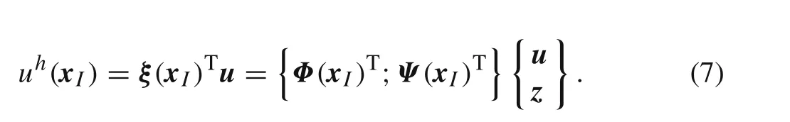
The RPIM shape functions are obtained using the Radial Point Interpolators(RPI),which combine a radial basis function,r(x)={r1(x),r2(x),...,rn(x)}T,with a polynomial basis function,p(x)={p1(x),p2(x),...,pm(x)}Twithmmonomial terms.Thus,the interpolation functionu h(x)can be defined at the interest pointx I∈?2by

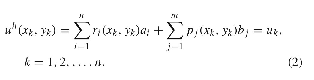
The inclusion of the following polynomial term is an extra requirement that guarantees unique approximation[5,17],

The computation of the shape functions is written in a matrix form as

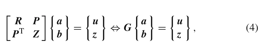
whereGis the complete moment matrix,Zis a null matrix defined byZ ij= 0,?{{i,j}∈N:{i,j}≤m},and the null vectorzcan be represented byzi= 0,?{i∈N:i≤m}.The vector for function values is defined asu i=u(xi),?{i∈N:i≤n}.The radial moment matrixRis represented as:Rij=ri(x j,y j)and the column vectorPas:P j=1.Since the distance is direction less,ri(x j,y j)=r j(xi,yi),i.e.,Rij=R ji,matrixRis symmetric.A unique solution is obtained if the inverse of the radial moment matrixRexists:?a b?T=G?1?u z?Tand the solvability of this system is usually guaranteed by the requirements rank(p)=m≤n[5,17].The influence-domain will always possess enough nodes to largely satisfy the previously mentioned condition.It is possible to obtain the interpolation with

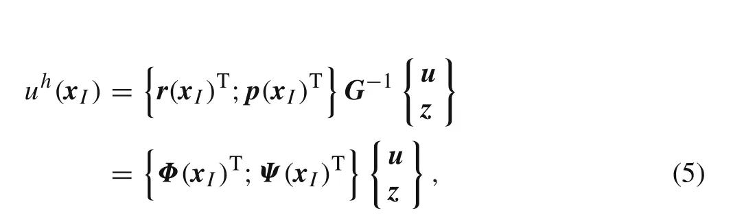
where the interpolation function vectorΦ(x I)and the residual vectorΨ(x I),with no relevant physical meaning,are expressed as follows

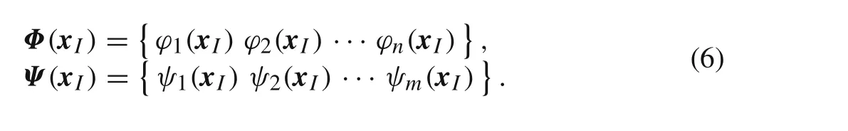
Being the field interpolation defined as

The spatial partial derivatives of the RPI shape functions are easily obtained,as showed in previous works[5,13].Additionally,it is possible to understand that the RPI test functionsΦ(x I)depend uniquely on the distribution of scattered nodes[5].Previous works[5,13,17]showed that RPI test functions possess the Kronecker delta property.Since the obtained RPI test functions have a local compact support it is possible to assemble a well-conditioned and a banded stiffness matrix.Furthermore,if a polynomial basis is included,the RPI test functions have reproducing properties and possess the partition of unity property[5].

3 Discrete equations system

3.1 Hooke law

In this study,the 3D solid domain is reduced to a 2D geometric representation.Therefore,a 2D deformation theory is assumed—the plane stress deformation theory—in which the 2D displacement field can be represented as follows

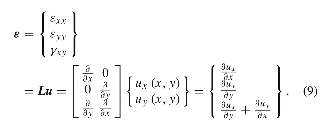
The corresponding deformation field is computed with

According to the Hooke’s law,it is possible to determine the stress field with the expression:

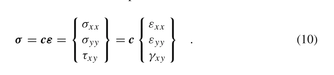
Notice thatcis the material constitutive matrix defined as follows

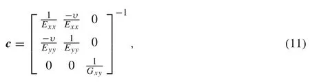
in whichE iiis the Young’s modulus in directioni,υijis the Poisson’s ratio,representing the ratio between the lateral contraction of a specimen in directioniwhen the specimen is stressed uniaxially in directionj.The shear modulus is defined byG xyand represents the variation angle between directionsiandj.

3.2 Weak-form of Galerkin

The discrete equation system is obtained using the Galerkin weak form.The Lagrangian functional is defined by

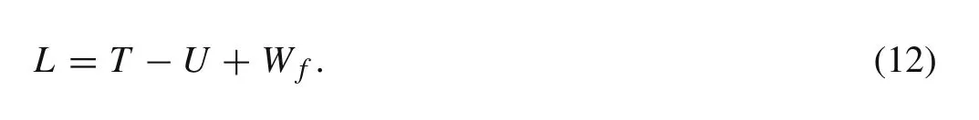
In the above relation,TandUare the kinetic and strain energy values respectively whileW fis known as the work produced by external forces.Afterwards,based on Hamilton’s principle and neglecting the dynamic effect,the minimization of the Lagrangian functional,δL=0,leads to the Galerkin weak form of the equilibrium equation:

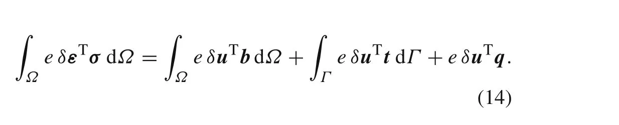
Beingbthe body force vector,tis the external traction force vector applied on a close surfaceSt,andqrepresents the external force vector applied on a close curveC q.Besides,it is worth nothing that dΛ=dxdydz.Since the beam shows a constant thickness,e,the integration domain can be reduced to a 2D simplification:dΩ=edxdy.Thus,the weak form of Galerkin can be re-written as

In the RPIM,the weak form has local support,which means that the discrete system of equations is developed firstly for every influence-domain.Then,the local systems of equations are assembled to form the global system of equations,which is solved afterwards.The RPIM trial function is given by Eq.(5).Thus,for each degree of freedom it is possible to write:

In the abovementioned equations,?i(xI)represents the RPIM interpolation function whileu x(xi)andu y(xi)are the nodal parameters of theith node belonging to the nodal set defined in the influence domain of the interest node ofxI.Subsequently,it is possible to generate a more general equation:

Furthermore,as a result of Eq.(5),it is possible to present developed form equation of the strain field:

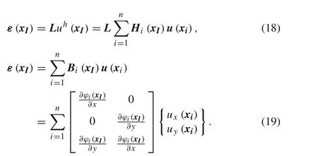
Fig.2 Example of a laminated composite beam of four layers,0?/90?/90?/0? under a uniform distributed load,b a punctual load applied at x=L,and c a punctual load applied at x=L/2

Notice thatBis the deformation matrix,which can be obtained with:B=LH.As mentioned before,the stress field is a function of strain vector.Thus,the developed relation of stress vector for an interest point(x I)could be written as follows

In order to compute the stiffness matrix,first it is necessary to present the general integration of the weak formulation for any interest point(x I):

In the end,it is possible to re-write Eq.(21)as a linear system of equations:

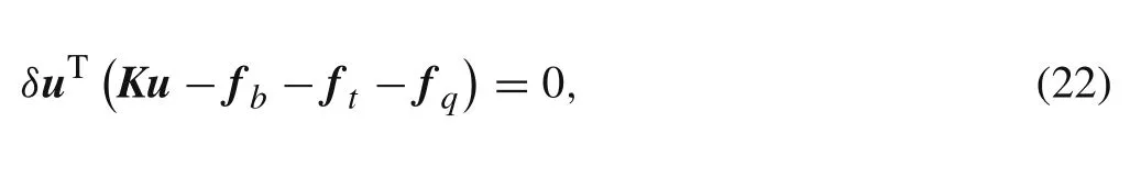
which leads to

Since the RPI test functions possess the delta Kronecker property,the essential boundary conditions are directly imposed in the global stiffness matrix.

4 Numerical examples

In this section,laminated composite beams are analysed using the RPIM meshless technique.In all presented examples,the mechanical properties of the laminated materialare:E1=25 MPa,E2=1 MPa,E3=1 MPa,G12=0.5 MPa,G23=0.2 MPa,G31=0.5 MPa,andυij=0.25,?{i,j} ∈{1,2,3}.If the material axis of the laminated are parallel to the Cartesian axis system,O123//Oxyz,the orientation of the laminated layer is 0?.If the material axisO2is parallel to the Cartesian axisO xand the material axisO1is parallel to the Cartesian axisOz,the orientation of the laminated layer is 90?.In this work,the laminates are always rotated around theO yaxis.

Here,the laminated beams are analysed considered three distinct boundary conditions:(1)clamped-free beam(CF),which is equivalent to the cantilever beam;(2)clamped–clamped beam(CC);and(3)hinged–hinged beam(HH),which is a simply supported beam.

Regarding the loading conditions,in this work two different loading conditions are assumed.A uniform distributed load along the beam mid-layerqo=1 N/m,as Fig.2a shows,and a concentrated loadQ o=1 N,assumingqo=1/eN/m andQ o=qo·e,applied in the end of the beam for the case of the CF beam,as Fig.2b shows,or applied in the centre of the beam for the CC and HH cases,as represented in Fig.2c.

Concerning the studied academic beam geometries,taking the example shown in Fig.2,all the geometries assume a constant uniform unit thickness and height,e=h=1 m.However,beams with distinct lengths are analysed,allowing the following ratios:L/h=10,L/h=20,andL/h=100.

Additionally,in this work,only regular nodal distributions are assumed.Thus,in Fig.3 are presented some examples of nodal distributions.The discretization used for theL/h=100 geometry are not represented in Fig.3 since those nodal distributions are very tight and the nodal spacing is not perceptible.

Additionally,in this study,the obtained punctual displacements are normalized by the expression,

following the recommendation of Ref.[23].For the HH and CC beams,the punctual displacement presented in the following subsections is always obtained in the geometric placex=L/2.For the CF beams;the punctual displacement presented in this work are always obtained inx=L.

Fig.3 Examples of Nodal distributions used in the analysis.a 41×5 nodes(205 nodes)for a L/h=10 2D geometry.b 81×9 nodes(729 nodes)for a L/h=10 2D geometry.c 41×3 nodes(123 nodes)for a L/h=20 2D geometry.d 81×5 nodes(405 nodes)for a L/h=20 2D geometry

4.1 Conversion study

In order to understand the accuracy and efficiency of the RPIM,a convergence study is performed.Thus,several distinct beams were analysed.First,a beam with a geometrical ratioL/h=10 was studied.For which,three distinct material distributions were assumed:a homogeneous beam with one single laminated layer with 0?(orthotropic beam 0?);a homogeneous beam with one single laminated layer with 90?(orthotropic beam 90?);and a beam with four laminated layers 0?/90?/90?/0?.Additionally,each one of the previous beams was submitted to different support conditions:HH;CC;and CF.Furthermore,all the previous mentioned beams were submitted to two load cases:a uniform distributed load and a concentrated load(as already mentioned in the introduction of this section).

The solid domain of the beam was discretized with the following nodal distributions:{21×3;41×5;81×9;161×17;301×31},which permits the corresponding total number of nodes:{63;205;729;2737;9331}.With these nodal distributions it was obtained the results presented in Figs.4 and 5 for the transverse normalized displacement for punctual and distributed load respectively.

Second,a beam with a geometrical ratioL/h=20 was analysed.All the previous considerations were once again assumed:material distributions(orthotropic beam 0?;orthotropic beam 90?;and laminated beam 0?/90?/90?/0?);boundary conditions(HH;CC;CF);loads conditions(uniform distributed and punctual load).Allowing to analyse 18 new beams.In order to perform the convergence study,new nodal distributions were considered:{41×3;81×5;161×9;321×17;401×21},leading to{123;405;1449;5457;8421}nodes correspondingly.The obtained punctual transverse normalized displacements are represented in Figs.4 and 5.

Fig.4 Convergence results of beams submitted to a puctualload.Boundary condition case:Clamp-free(a–c),Clamp–clamp(d–f),Hinged–hinged(g–i).Material distribution:orthotropic beam 0? (a,d,g),orthotropic beam 90? (b,e,h),laminated beam 0?/90?/90?/0? (c,f,i)

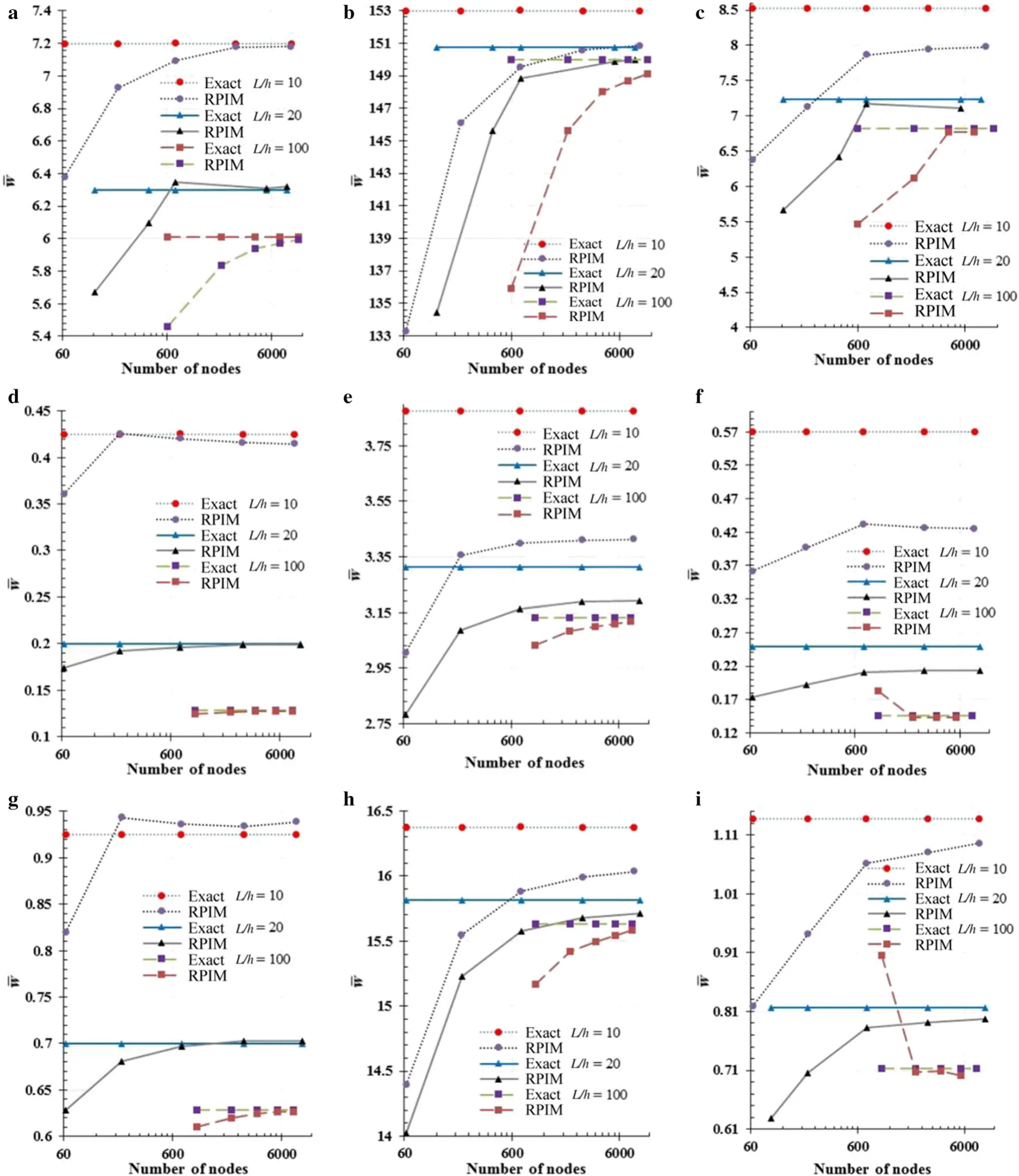
Fig.5 Convergence results of beams submitted to a distributed load.Boundary condition case:Clamp-free(a–c),Clamp–clamp(d–f),Hinged–hinged(g–i).Material distribution:orthotropic beam 0? (a,d,g),orthotropic beam 90? (b,e,h),laminated beam 0?/90?/90?/0? (c,f,i)

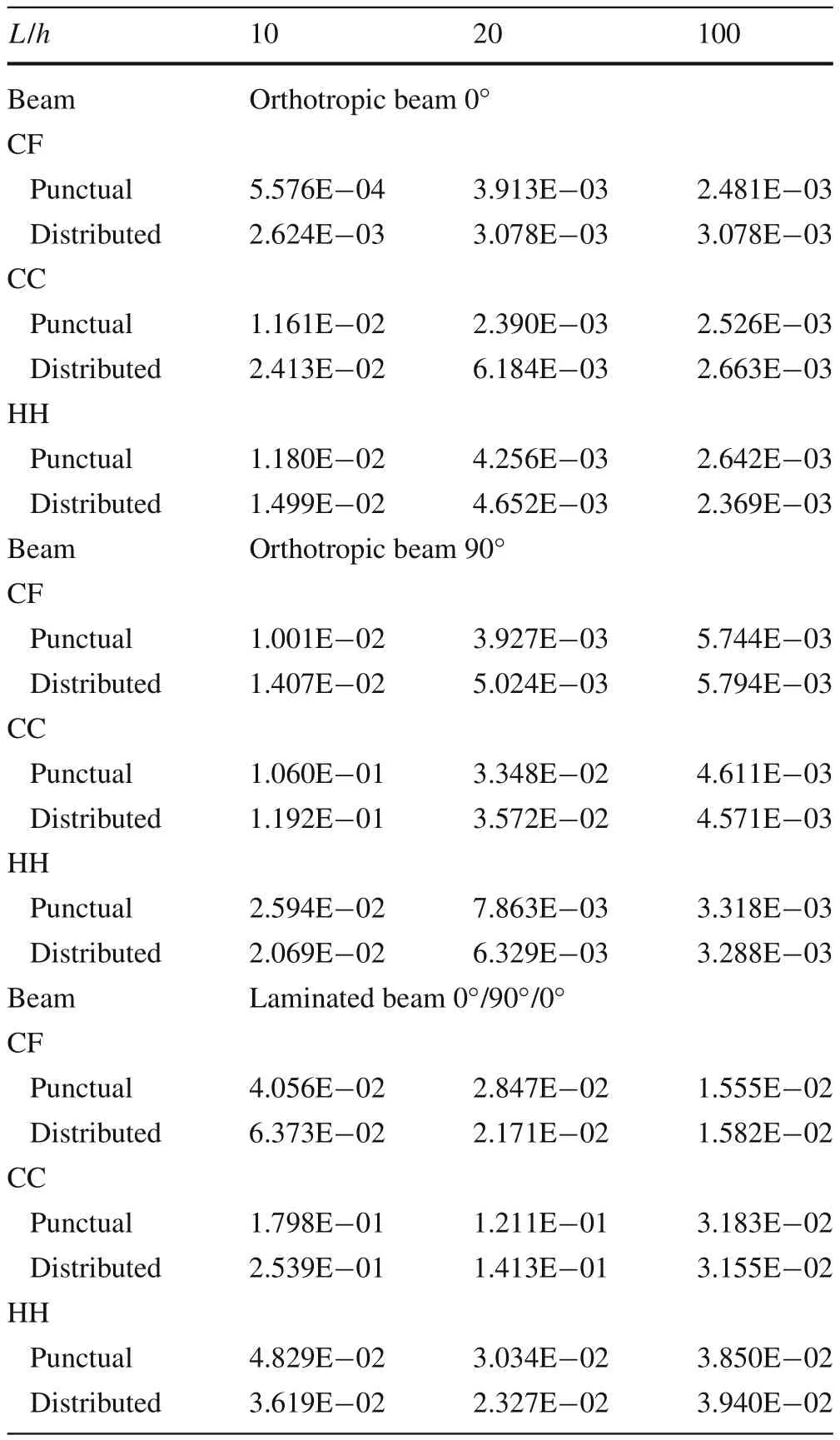
Table 1 Errors with respect to the exact analytical solution

The last convergence study regards a beam with a geometrical ratioL/h=100.Similarly to the last analysis,the same previous material distributions,boundary conditions and loading conditions were considered.Since the geometry of the beam has changed,new nodal distributions were generated:{201×3;401×5;601×7;901×9;1001×11},corresponding to{603;2005;4207;7209;11011}nodes.The results are once again plotted in Figs.4 and 5,allowing a straightforward comparison with the previous convergence studies.

As Figs.4 and 5 show,the RPIM allows to obtain results very close with the exact solution.Nevertheless,in some examples,the RPIM solution appears to have some difficulty to reach the analytical solution,showing a slower convergence rate.This phenomenon can be explain with the fact that the RPIM generally cannot pass the standard path test and guarantee monotonic convergence[27].However,thisissue has been successfully solved combining the gradient(strain)smoothing technique with the RPIM—the smoothed RPIM(S-RPIM)[40].When compared with the classical RPIM and other traditional techniques,such as the FEM,the S-RPIM possesses a softened stiffness,allowing it:to pass the standard patch test,to show a high convergence rate,to solve the volumetric locking issue,to provide a upper bound solution,and to present a superior behaviour in the analysis of nonlinear problems[40–43].

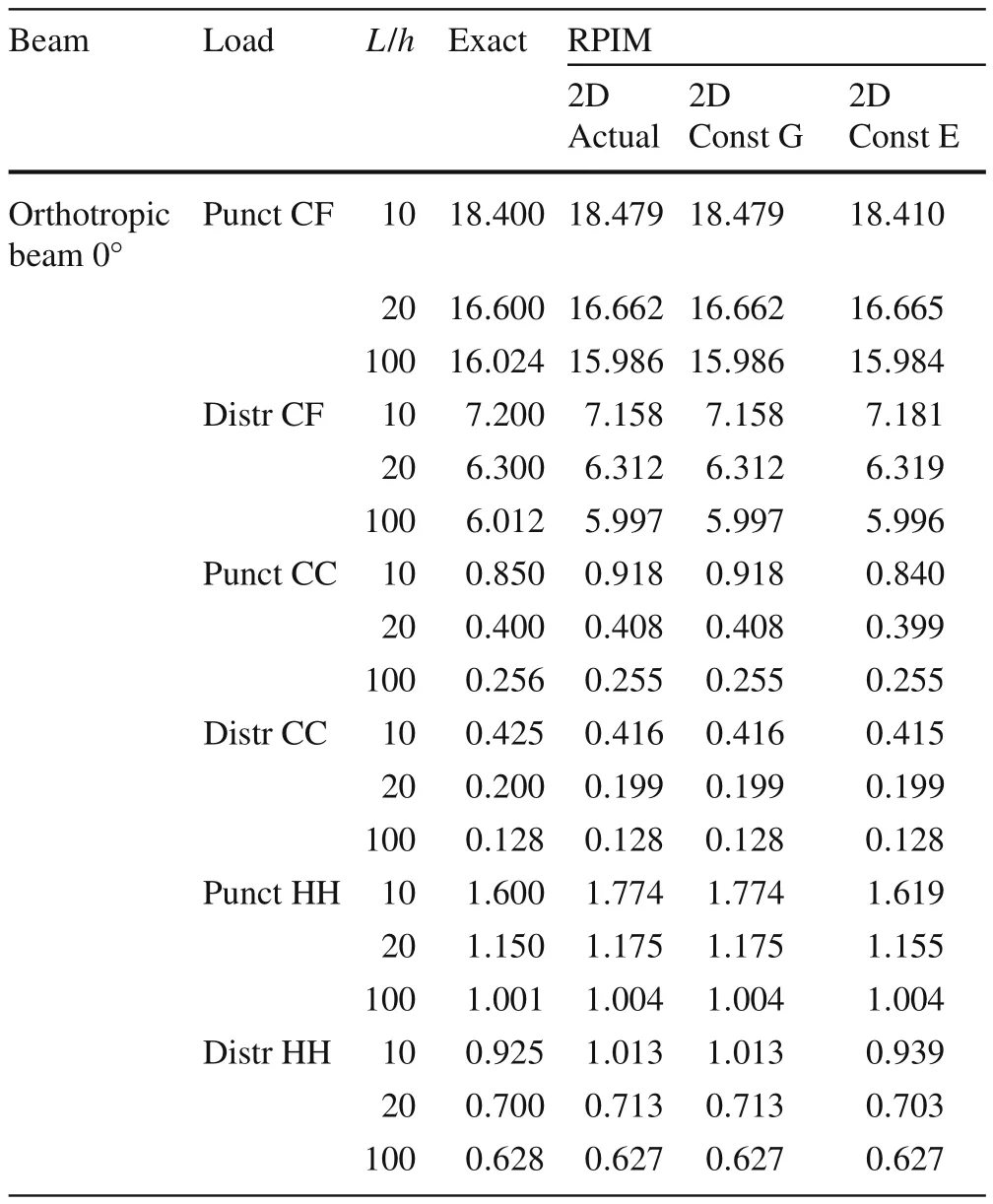
Table 2 Normalized displacements obtained with the RPIM and compared to exact solution for the orthotropic beam(0?)

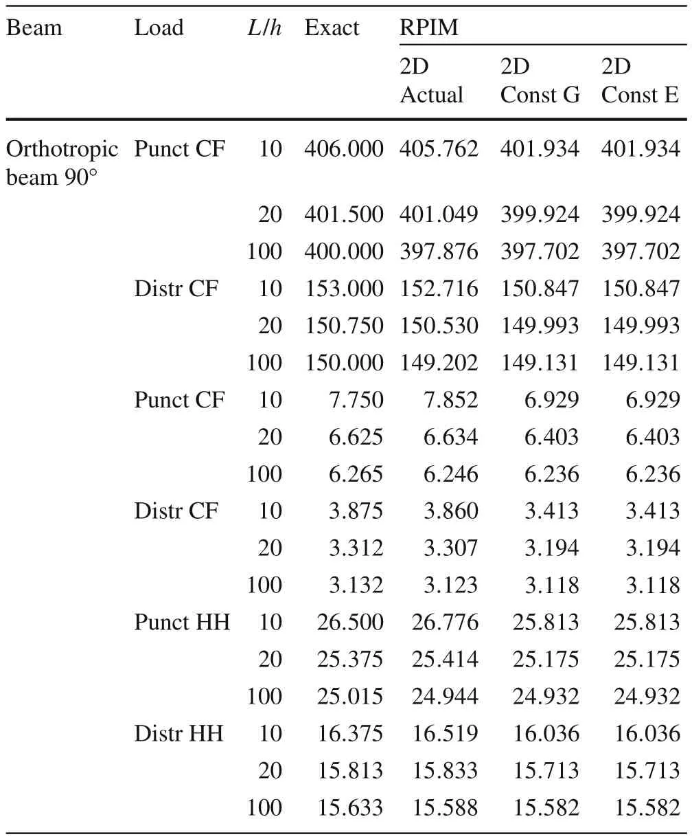
Table 3 Normalized displacements obtained with the RPIM and compared to exact solution for the orthotropic beam(90?)

In Table 1 are presented the punctual errors with respect to the exact solution,for each analysed example,considering the corresponding highest nodal distribution.In Tables 2,3,and 4 are presented the punctual transverse normalized displacements obtained with the highest nodal distribution for each analysed case.Notice that in those tables it appear three RPIM results.The results of column “RPIM 2D actual”regard the formulation presented in this manuscript.The values in column “RPIM 2D const G”are obtained consideringG12=G23=G31=0.5 MPa and the values in column “RPIM 2D const E”are obtained consideringE11=E33=25 MPa.

Notice that from Tables 2,3,and 4,it possible to compare the RPIM solutions with the exact solution.For instance,assuming beams with the boundary CF.For the orthotropic beam 0?,withL/h=10,and submitted to a punctual load,it is possible to achieve a solution error of only 0.055%.For the orthotropic beam 90?,withL/h=20,and submitted to an uniform distributed load,one obtained a solution error of 0.502%.And for the laminated beam 0?/90?/90?/0?,consideringL/h=100 and submitted to a uniform distributed load,one found a solution error of 1.582%.These features can be seen in Table 1.The error is calculated with the expression:|wRPIM?wexact|/|wexact|.

Additionally,a comparison test between the FEM and the RPIM was performed.Thus,for an orthotropic beam(90?),with the geometric ratioL/h=10,constrained by the boundary condition CF and submitted to a punctual load,it was conducted a new convergence test.The results regarding the punctual transverse normalized displacements are presented in Table 5.It is visible that the final converged solutions of FEM and RPIM are very close.However,the RPIM converge faster to the final solution.

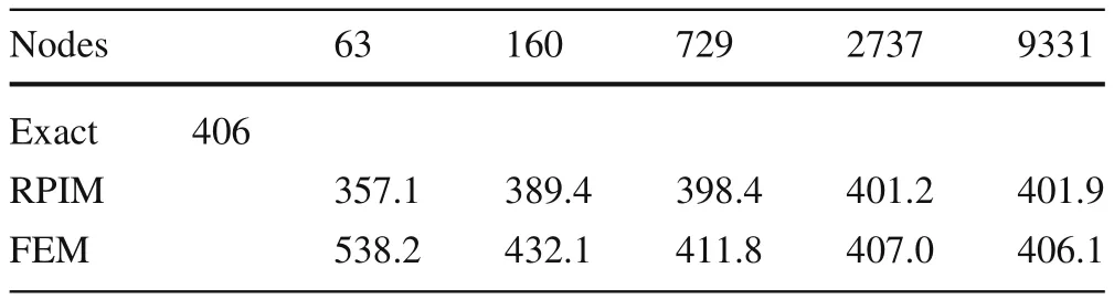
Table 5 Comparison between the RPIM and FEM solution for the CF orthotropic beam 90?(L/h=10)

4.2 Stresses analysis

Here,it is performed a stress analysis of the several beams presented in the previous subsection.Thus,considering the boundary condition CF,three distinct material distributions were assumed:orthotropic beam 0?;orthotropic beam 90?;and laminated beam 0?/90?/90?/0?.Additionally,all the three geometric ratios were considered in the study:L/h={10,20,100},beingh=0.1 m.In Fig.6 it is shown the stress distribution along the thickness of each analysed beam,considering a punctual load,and in Fig.7 the same representation can be found for the uniform distributed load case.The presented stresses(σxx,σyy,τxy)were obtained in the clamped face of the beam,x=0 m.

The stress distribution along the thickness of the beam is in accordance with the stress distribution obtained with high order shear deformation theories for plates under transversal loads.It is possible to observe the effect of introducing layers wit 90?orientation:the stress lever in those layers.

Afterwards,the same procedure was repeated assuming a CC boundary condition.Once again,all the previous considerations were applied:three material distributions(orthotropic beam 0?;orthotropic beam 90?;and laminated beam 0?/90?/90?/0?);three geometric configurationsL/h={10,20,100}withh=0.1 m;and two load cases(punctual load and uniform distributed load).

The results concerning the punctual load are presented in Fig.8 the solution for the uniform distributed load are shown in Fig.9.Likewise,in this study the presented stresses(σxx,σyy,τxy)were obtained in the clamped face of the beamx=0.As in the previous case,the stress distribution agrees with the stress distribution predicted by equivalent single layer theories for plates.

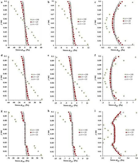
Fig.6 Stresses in cross section for clamp-free beams,under punctual load.Material distribution:orthotropic beam 0? (a–c).Orthotropic beam 90? (d–f).Laminated beam 0?/90?/90?/0? (g–i).Stresses:σxx(a,d,g),σyy(b,e,h),σxy(c,f,i)

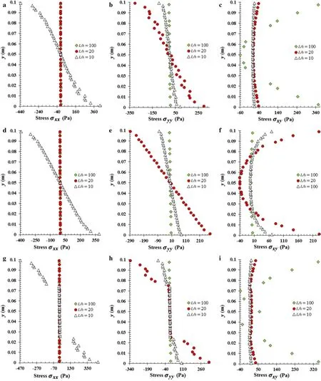
Fig.7 Stresses in cross section for clamp-free beams,under distributed load.Material distribution:orthotropic beam 0? (a–c).Orthotropic beam 90? (d–f).Laminated beam 0?/90?/90?/0? (g–i).Stresses:σxx(a,d,g),σyy(b,e,h),σxy(c,f,i)

Fig.8 Stresses in cross section for clamp-clamp beams,under punctual load.Material distribution:orthotropic beam 0? (a–c).Orthotropic beam 90? (d–f).Laminated beam 0?/90?/90?/0? (g–i).Stresses:σxx(a,d,g),σyy(b,e,h),σxy(c,f,i)

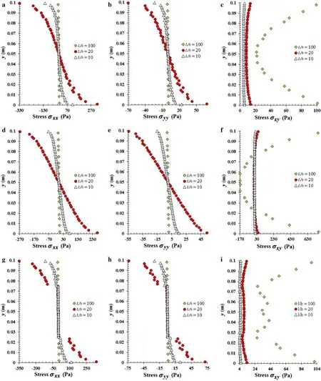
Fig.9 Stressesin cross section for clamp–clamp beams,under distributed load.Material distribution:orthotropic beam 0? (a–c).Orthotropic beam 90? (d–f).Laminated beam 0?/90?/90?/0? (g–i).Stresses:σxx(a,d,g),σyy(b,e,h),σxy(c,f,i)

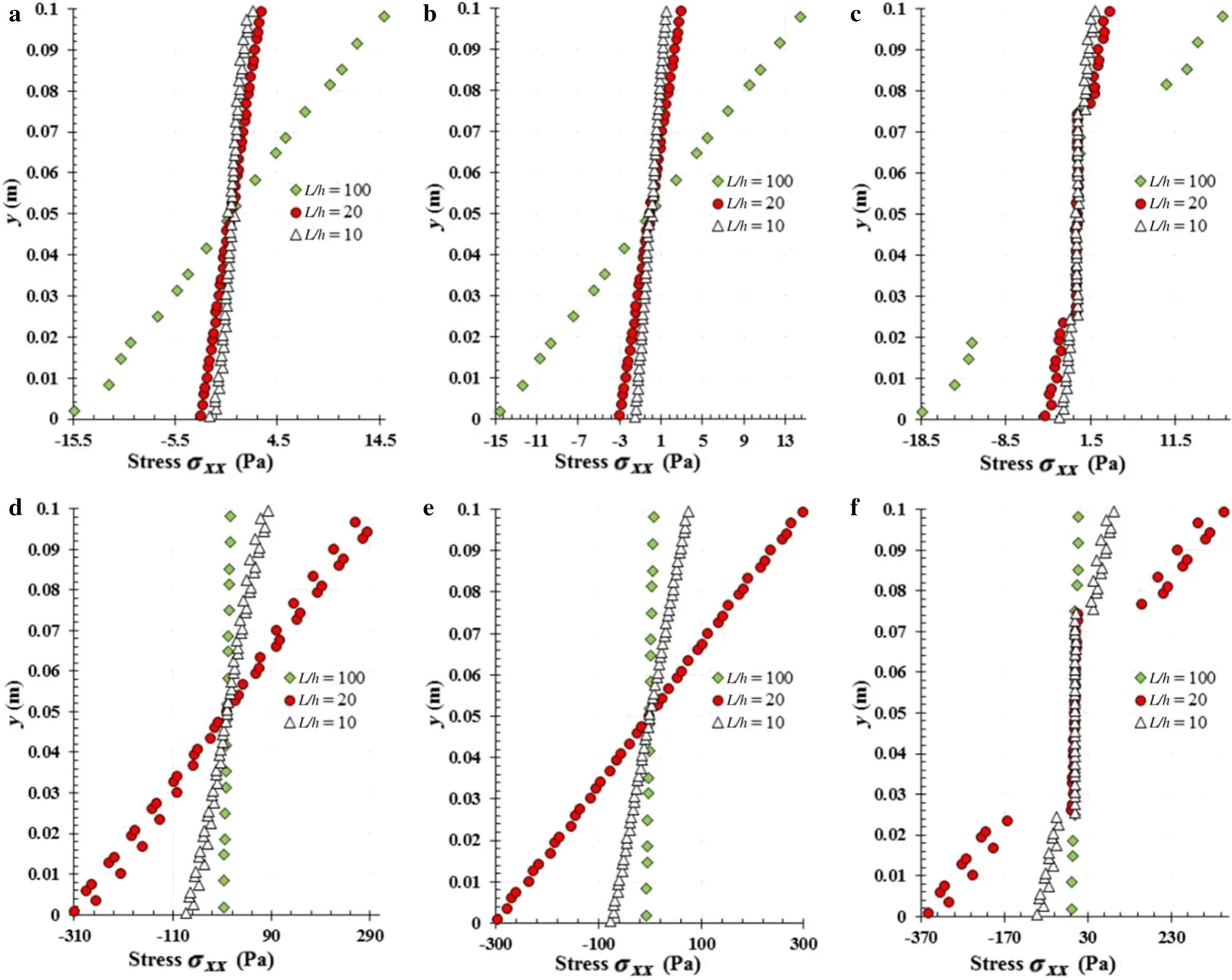
Fig.10 Stresses forces effecting in cross section y for hinged–hinged beam due to punctual load in a–c and distributed load in d–f.Material distribution:orthotropic beam 0? (a,d),orthotropic beam 90? (b,e),laminated beam 0?/90?/90?/0? (c,f)

Finally,the HHboundary condition was studied.As in previous analyses,three beamgeometries were assumed:L/h={10,20,100}withh=0.1 m,having each one the three material distributions already presented:orthotropic beam 0?;orthotropic beam90?;and laminated beam0?/90?/90?/0?.Similar to the previous analyses,two load cases were applied:a punctual load and an uniform distributed load.The results regarding the normal stressσxx,which are presented in Fig.10,were obtained in the centre of the beam,x=L/2.It is possible to observe,as expected,that the type of the load leads to distinct stress distributions along the beam thickness.

5 Conclusions

In this work a 2D deformation theory was combined with an efficient meshless method to analyse composite laminated beams under several essential and natural boundary conditions.Although several meshless methods are available in the literature,not all of them are robust and accurate.In this study,the authors decided to use a popular and highly efficient meshless method,which allies an easy computational effort with a robust performance:the RPIM.Thus,the authors have written a complete RPIM code,prepared to analyse composite laminated beam using a 2D numerical approach.This procedure permits a more assertive comparison with other numerical techniques,such as the FEM.

In this work,several composite laminated beams were analysed.Notice that all the following alternatives were here considered in the present study:three material distributions(orthotropic beam 0?;orthotropic beam 90?;and laminated beam 0?/90?/90?/0?);three essential boundary conditions(hinged–hinged;clamped–clamped;clamped-free);two loads cases(punctual load;uniform distributed load);three geometric configurations(L/h={10;20;100});and at least 5 nodal meshes per geometry.Which leads,at least,to a total of 270 beams analysed.This significant amount of studies permit to understand better the RPIM behaviour in the analysis of 2D numerical models with distinct anisotropic materials,possessing material discontinues.

Generally,the RPIM was capable to produce numerical solution always very close with the available analytical solution,regardless the kind of beam analysed.The most significant advantage of the RPIM is its computational cost.The RPIM permits to obtain accurate results within a reduced computation time and it possess a high convergence rate,which allows to achieve the final converged solution faster than the FEM.Another advantage of the RPIM is the smoothness of the obtained variable fields.The stress and strain fields,besides being accurate,are very smooth,which permits to expect excellent numerical behaviour in nonlinear analysis(elasto-plasticity;damage).

Additionally,the numerical approach here proposed has advantages when compared with equivalent single layer theories,since this approach permits to study delamination phenomena,fracture and damage occurrences along the laminate thickness and between layers.In the present work,these problems were not addressed,however the obtained results(at the stress distribution)allow to expect that the RPIM will be capable to simulate these phenomena with more efficiency than other discretization techniques available in the literature.

This work permits to conclude that the RPIM is an efficient alternative discretization technique capable to analyse 2D laminated beams under several essential and natural boundary conditions.

AcknowledgementsThe authors truly acknowledge the funding provided by Ministério da Ciência,Tecnologia e Ensino Superior—Funda??o para a Ciência e a Tecnologia(Portugal)(Grants SFRH/BPD/75072/2010,SFRH/BPD/111020/2015),and by the inter-institutional projects from LAETA(GrantUID/EMS/50022/2013).Additionally,the authors gratefully acknowledge the funding of Project NORTE-01-0145-FEDER-000022—SciTech—Science and Technology for Competitive and Sustainable Industries,cofinanced by Programa Operacional Regionaldo Norte(GrantNORTE2020),through Fundo Europeu de Desenvolvimento Regional(FEDER).

1.Reddy,J.N.:Mechanics of Laminated Composite Plates and Shells:Theory and Analysis,2nd edn.CRC Press LLC,Boca Raton(2003)

2.Reddy,J.N.,Miravete,A.:Practical Analysis of Composite Laminates.CRC Press LLC,Boca Raton(1995)

3.Nguyen,V.P.,Rabczuk,T.,Bordas,S.,et al.:Meshless methods:a review and computer implementation aspects.Math.Comput.Simul.79,763–813(2008)

4.Belytschko,T.,Krongauz,Y.,Organ,D.,et al.:Meshless methods:an overview and recent developments.Comput.Methods Appl.Mech.Eng.139,3–47(1996)

5.Belinha,J.:Lecture Notes in Computational Vision and Biomechanics,vol.16.Springer,Dordrecht(2014)

6.Gingold, R.A., Monaghan, J.J.: Smoothed particle hydrodynamics—theory and application to non-spherical stars.Mon.Not.R.Astron.Soc.181,375–389(1977)

7.Randles,P.W.,Libersky,L.D.:Smoothed particle hydrodynamics:some recent improvements and applications.Comput.Methods Appl.Mech.Eng.139,375–408(1996)

8.Nayroles,B.,Touzot,G.,Villon,P.:Generalizing the finite element method:diffuse approximation and diffuse elements.Comput.Mech.10,307–318(1992)

9.Lancaster,P.,Salkauskas,K.:Surfaces generated by moving least squares methods.Math.Comput.37,141–141(1981)

10.Belytschko,T.,Lu,Y.Y.,Gu,L.:Element-free Galerkin methods.Int.J.Numer.Methods Eng.37,229–256(1994)

11.Liu,W.K.,Jun,S.,Li,S.,et al.:Reproducing kernel particle methods for structural dynamics.Int.J.Numer.Methods Eng.38,1655–1679(1995)

12.Atluri,S.N.,Zhu,T.:A new meshless local Petrov–Galerkin(MLPG)approach in computational mechanics.Comput.Mech.22,117–127(1998)

13.Dinis,L.M.J.S.,Natal Jorge,R.M.,Belinha,J.:Analysis of 3D solids using the natural neighbour radial point interpolation method.Comput.Methods Appl.Mech.Eng.196,2009–2028(2007)

14.Liew,K.M.,Zhao,X.,Ferreira,A.J.M.:A review of meshless methods for laminated and functionally graded plates and shells.Compos.Struct.93,2031–2041(2011)

15.Liu,G.R.,Gu,Y.T.:A point interpolation method for two dimensional solids.Int.J.Numer.Methods Eng.50,937–951(2001)

16.Wang,J.G.,Liu,G.R.,Wu,Y.G.:A point interpolation method for simulating dissipation process of consolidation.Comput.Methods Appl.Mech.Eng.190,5907–5922(2001)

17.Wang,J.G.,Liu,G.R.:A point interpolation meshless method based on radial basis functions.Int.J.Numer.Methods Eng.54,1623–1648(2002)

18.Wang,J.G.,Liu,G.R.:On the optimal shape parameters of radial basis functions used for 2-D meshless methods.Comput.Methods Appl.Mech.Eng.191,2611–2630(2002)

19.Braun,J.,Sambridge,M.:A numerical method for solving partial differential equations on highly irregular evolving grids.Nature 376,655–660(1995)

20.Sukumar,N.,Moran,B.,Semenov,A.Y.,et al.:Natural neighbour Galerkin methods.Int.J.Numer.Methods Eng.50,1–27(2001)

21.Idelsohn,S.R.,O?ate,E.,Calvo,N.,et al.:The meshless finite element method.Int.J.Numer.Methods Eng.58,893–912(2003)

22.Dinis,L.M.J.S.,Jorge,R.M.N.,Belinha,J.:Analysis of plates and laminates using the natural neighbour radial point interpolation method.Eng.Anal.Bound.Elem.32,267–279(2008)

23.Moreira,S.,Belinha,J.,Dinis,L.M.J.S.,et al.:Análise de vigas laminadas utilizando o natural neighbour radial point interpolation method.Rev.Int.Métodos Numéricos para Cálculo y Dise?o en Ing.30,108–120(2014)(in Portuguese)

24.Belinha,J.,Dinis,L.M.J.S.,Jorge,R.M.N.:The natural radial element method.Int.J.Numer.Methods Eng.93,1286–1313(2013)

25.Belinha,J.,Dinis,L.M.J.S.,Jorge,R.M.N.:Analysis of thick plates by the natural radial element method.Int.J.Mech.Sci.76,33–48(2013)

26.Belinha,J.,Dinis,L.M.J.S.,Jorge,R.M.N.:Composite laminated plate analysis using the natural radial element method.Compos.Struct.103,50–67(2013)

27.Liu,G.R.:Mesh Free Methods,Moving beyond the Finite Element Method,2nd edn.CRC Press LLC,Boca Raton(2009)

28.Liu,G.R.,Gu,Y.T.:An Introduction to Meshfree Methods and Their Programming.Springer,Dordrecht(2005)

29.Belinha,J.,Araújo,A.L.,Ferreira,A.J.M.,et al.:The analysis of laminated plates using distinct advanced discretization meshless techniques.Compos.Struct.143,165–179(2016)

30.Schaback,R.:Error estimates and condition numbers for radial basis function interpolation.Adv.Comput.Math.3,251–264(1995)

31.Wendland,H.:Error estimates for interpolation by compactly supported radial basis functions of minimal degree.J.Approx.Theory 93,258–272(1998)

32.Gu,Y.T.,Liu,G.R.:A local point interpolation method for static and dynamic analysis of thin beams.Comput.Methods Appl.Mech.Eng.190,5515–5528(2001)

33.Liu,G.R.,Gu,Y.T.:A local radial point interpolation method(LRPIM)for free vibration analyses of 2-D solids.J.Sound Vib.246,29–46(2001)

34.Liu,G.R.,Yan,L.,Wang,J.G.,et al.:Point interpolation method based on local residual formulation using radial basis functions.Struct.Eng.Mech.14,713–732(2002)

35.Liu,G.R.,Chen,X.L.:A mesh free method for static and free vibration analysis of thin plates of arbitrary shape.J.Sound Vib.241,839–855(2001)

36.Liu,L.,Liu,G.R.,Tan,V.B.C.:Element free method for static and free vibration analysis of spatial thin shell structures.Comput.Methods Appl.Mech.Eng.191,5923–5942(2002)

37.Liu,G.R.,Dai,K.Y.,Lim,K.M.,et al.:A point interpolation mesh free method for static and frequency analysis of two-dimensional piezoelectric structures.Comput.Mech.29,510–519(2002)

38.Liu,G.R.,Zhang,G.Y.,Gu,Y.T.,et al.:A meshfree radial point interpolation method(RPIM)for three-dimensional solids.Comput.Mech.36,421–430(2005)

39.Wang,J.,Liu,G.,Lin,P.:Numerical analysis of Biot’s consolidation process by radial point interpolation method.Int.J.Solids Struct.39,1557–1573(2002)

40.Liu,G.-R.,Zhang,G.-Y.:Smoothed Point Interpolation Methods:G Space Theory and Weakened Weakforms.World Scientific,Singapore(2013)

41.Zhang,G.Y.,Li,Y.,Gao,X.X.,et al.:Smoothed point interpolation method for elastoplastic analysis.Int.J.Comput.Methods 12,1540013(2015)

42.Liu,G.R.,Zhang,G.Y.,Zong,Z.,et al.:Meshfree cell-based smoothed alpha radial point interpolation method(CS-αRPIM)for solid mechanics problems.Int.J.Comput.Methods 10,1350020(2013)

43.Zhang,G.Y.,Liu,G.R.,Nguyen,T.T.,et al.:The upper bound property for solid mechanics of the linearly conforming radial point interpolation method(LC-RPIM).Int.J.Comput.Methods4,521–541(2007)