Using Generalized Poisson Distribution to Model the Patterns of Species Abundances in Three Layers of South Subtropical Forest
2022-03-11 09:51:44YINZuoyun
生態(tài)環(huán)境學報 2022年1期
YIN Zuoyun
1. College of Horticulture and Landscape Architecture, Zhongkai University of Agriculture and Engineering, Guangzhou 510230, P. R. China;
2. Guangdong Forest Research Institute (Guangdong Academy of Forestry), Guangzhou 510520, P. R. China;
3. South China Botanical Garden of the Chinese Academy of Sciences, Guangzhou 510650, P. R. China
Abstract: The species abundance distribution (SAD) in a biological community showed typical inverse J-shaped pattern, and the SAD modelling study was contributed to solve practical problems such as the species configuration in forest ecological restoration. This study examines whether a discrete distribution with over-dispersion (i.e., variance>mean), the generalized Poisson (GP) distribution with two parameters, λ and α, can describe the SAD pattern, and whether its parameters are related to community species diversity by using the data from the three layers of a lower subtropical mixture forest in Dinghushan Biosphere Reserve, South China. The results showed that the observed SADs for all three layers of the forest showed similar inverse J-shaped distribution curves and followed the zero-truncated GP, with significantly decreasing λ and slightly increasing α from the tree, shrub to herb layer in the community. The parameter α better reflected the species diversity than λ, and thus the former could serve as a measure of the species diversity in a community. Comparisons between the GP and the Poisson lognormal (PLN) distribution showed that the former better fitted the SAD datasets than the latter for three layers. Therefore, the GP better estimated the potential species richness in the community. The GP distribution was more suitable to model the observed SAD with over-dispersed count data than the PLN, and thus the former might have a wider application prospect than the latter, especially in the estimation of the potential species richness in a community as well as on a local or regional scale and the determination of the species proportion for ecological restoration of degraded forests.
Keywords: species abundance distribution (SAD); generalized Poisson distribution; Poisson lognormal distribution; forest layers;maximum likelihood method
The species abundance distribution (SAD) in a biological community follows one of ecology’s oldest and most universal laws, that is, every community shows a hollow or hyperbolic shape (i.e., inverse J-shape) with many rare species and a few common species (McGill et al., 2007; Yin et al., 2018; Aziz et al., 2020). The distribution of commonness and rarity among species, firstly described by Preston (1948), has often been regarded as one of the best-documented patterns in natural communities (Molles, 1999; Yin et al., 1999; McGill et al., 2007; Yin et al., 2018). The SAD pattern was so fundamental that Sugihara (1980)referred to it as “minimal community structure”. He et al. (2002) stated that the area, abundance, richness, and spatial distribution of species have been central components of community ecology. In recent years,SADs have received more attention, and the“community” has been extended to “multispecies collection” in a specific spatio-temporal condition(Peng et al., 2003; Yin, 2005; Yin et al., 2018; Aziz et al., 2020). Moreover, the quantitative studies on the patterns and dynamics of a natural forest community,especially the SAD modeling, can help solve practical problems such as the species selection and configuration in the reconstruction of forest vegetation(Zeng et al., 2013; Xian et al., 2014; Yin, 2018; Yin et al., 2018; Villa et al., 2019; Aziz et al., 2020; Chen et al., 2020; An et al., 2021).
Modeling SAD, however, has not been straightforward. Ecologists have developed various statistical and niche distribution models (McGill et al.,2007), mainly including the lognormal (Preston, 1948)and Poisson lognormal (PLN; Grundy, 1951). Each of these models has some unique characteristics which may fit the SAD data in different types of biological communities (Peng et al., 2003). Among these, Preston’s lognormal distribution has been most widely used to fit a variety of SAD data from surprisingly diverse plant and animal communities or collections (Whittaker, 1965;Slocomb et al., 1977; Miller et al., 1989; Brown et al.,1995; Engen, 2001; Fesl, 2002; McGill, 2003; Yin et al.,2005a; Yin et al., 2018).
The lognormal is a continuous distribution in statistics. However, the abundance of a species or the number of individuals of the species (often expressed as r) is apparently a discrete variable (count data).Preston (1948) expressed the abundances in relative terms and the SAD as a frequency distribution by grouping r on a log2scale (called the “octave”) and proposed to fit the lognormal distribution. He treated the observed SAD as a truncated, grouped lognormal distribution (Preston, 1948; Yin et al., 2009). However,such statistical treatments adopt somewhat arbitrary abundance grouping and often ignore the effect of Poisson sampling variability (Bulmer, 1974; Kempton,1974). Furthermore, this method does not provide a satisfactory approximation to the probabilities, Pr,when r is near zero, as shown in Grundy (1951) and reiterated by Kempton et al. (1974). In any case, it should be reasonable to use some discrete probability distributions to model a count dataset where the abundance is a discrete variable. Ecologists have presented a mathematically more accurate compound distribution (i.e., discrete PLN) (Grundy, 1951; Bulmer,1974; Kempton et al., 1974; Pielou, 1977; Etienne et al., 2004; McGill et al., 2007). However, the PLN distribution is based on the assumption that the number of individuals per species (i.e., r) in the multispecies collection is a Poisson variate (Grundy, 1951; Bulmer,1974; Pielou, 1977). This assumption is often not realistic because in nature, individuals of most species are seldom random or regular but rather contagiously(i.e., in clumps) distributed through space (Greig-Smith, 1983; Brown et al., 1995; He et al., 1997; Condit et al., 2000; Yin et al., 2005b).
As an effort to overcome the limitations mentioned above, it is proposed to use another discrete probability distribution, the generalized Poisson (GP) distribution,without the PLN’s assuming a spatial Poisson distribution of each species. The GP distribution introduced by Consul et al. (1973) and investigated extensively by Consul (1989) has two parameters and is defined on the non-negative integers. It is a natural extension of the standard Poisson distribution with one parameter and has some unique properties (Tuenter,2000). It extends the Poisson by its ability to describe settings where the occurrence probability of a single event does not remain constant as in a Poisson process,but is influenced by previous occurrences. The GP could accurately describe the spatial distribution of insects,where initial occupation of a spot by an individual of a species has an impact on the attractiveness of the spot to other members of the species (Consul, 1989), and also describe the number of units of different commodities purchased by consumers, where current sales have an influence on the subsequent ones through repeat purchases (Tuenter, 2000). Similarly, based on the hypothesis that the abundance of a species should affect that of others, we used the GP to describe an inverse J-shaped SAD in a forest community. Since no species will have zero (or smaller than one) individuals in the sample,the distribution described here is zero-truncated.
To date, the GP distribution has not been reported to model the SAD in community ecology. Using an iterative likelihood method, we examine whether the discrete GP distribution fits well with the SAD count data in a forest community and whether the GP is better than another discrete distribution, the PLN,which integrates the commonly-used lognormal with the Poisson. We also examine whether the two parameters in GP can help assess species diversity in the forest community.
1 METHODS
1.1 Data Source
In accordance with the Smithsonian/MAB biodiversity program, a permanent forest community plot (100 m×100 m) was established in 1999 at an elevation of 250 m in Feitianyan of Dinghushan Biosphere Reserve (112°30′39″-112°33′41″E,23°09′21″-23°11′30″N), Guangdong Province, South China (for details, see also Zhang et al., 2002; Yin,2005). The community belongs to south subtropical evergreen needle- and broad-leaved mixed forest of around 70-80 years age. The tree layer was dominated by Castanopsis chinensis, Schima superba, and Pinus massoniana. The shrub layer had several dominant species such as Litsea rotundifolia var. oblongifolia,Psychotria rubra, and Rhodomyrtus tomentosa, and the herb layer was dominated by Lophatherum gracile. All the tree species with diameter at breast height (DBH)≥1 cm were censused in the tree layer of the community by dividing the 1 hm2plot into 25400 m2subplots.Within each subplot, a 25 m2quadrat was randomly chosen to record the shrubs and the seedlings of trees(DBH<1cm, height≥50 cm) in the shrub layer.Meanwhile, a 1 m2subquadrate was randomly selected in every 25 m2quadrat to survey the herbs and the seedlings of trees and shrubs (height<50 cm) in the herb layer.
1.2 Distribution model
Suppose that (1) the number of members(individuals) of the jth species in a collection (i.e., a forest community in this study) with S*species is a Poisson variate with a mean, λj(j = 1, 2, …, S*); and (2)the λj’s can be regarded as constituting S*independent observations from a LN distribution, that is, lnλjis normally distributed with the mean μ and the variance σ2. The probability that a randomly chosen species represented by r individuals in the collection is thus a discrete, compound PLN distribution with the probability function (Grundy, 1951, Bulmer, 1974;Pielou, 1977; Yin et al., 2005c):
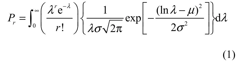
where r = 0, 1, 2, …, λ > 0, σ > 0, ∞ > μ > -∞.
Following Famoye (1993; see also Tuenter, 2000),the probability function Prof GP distribution is defined on the non-negative integers by
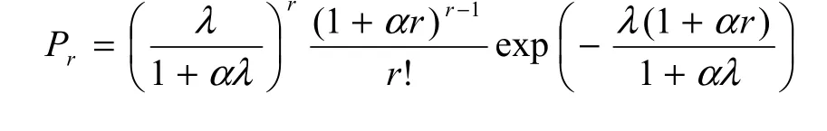
Thus, the GP distribution is a natural extension of standard Poisson distribution. If α=0, the probability function in Equation 2 reduces to the Poisson distribution with equidispersion, i.e. V=M, as indicated in Equations 3 and 4. If α>0, then V>M and the GP distribution represents count data with overdispersion(Wang et al., 1997).
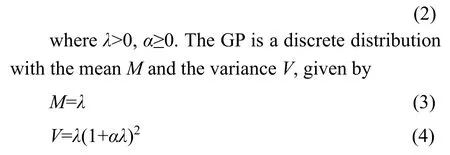
If λ→∞, then the complete GP distribution in Equation 2, is transformed into
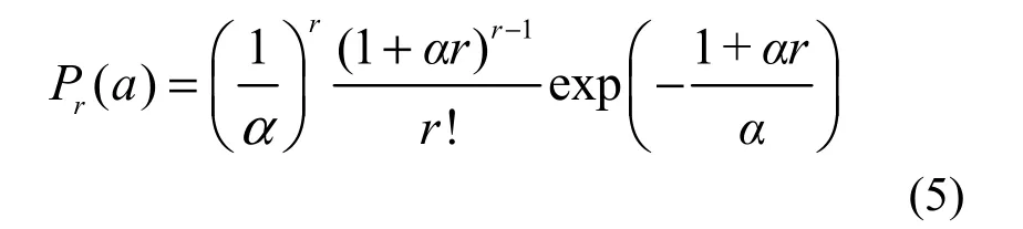
which is another discrete distribution with only one parameter α. This means that the individuals of one or more species are infinitely large in number, or completely sampled in the whole community according to Equation 3.
To model the SAD count data in a community with overdispersion, i.e. V>M, we can assume that the SAD in a community with total number of individuals N*and of species S*follows a complete GP distribution. There are the numbers of species S0, S1, S2, … with the numbers of individuals r=0, 1, 2, …, respectively, as such we get the expected number of species with r individuals (Pielou, 1977):
which is the number of species without any individuals (i.e., not collected in a sample; Pielou,1977).
However, the true value of S*is usually unknown because the expected numbers of individuals of some species are smaller than 1 and such species are basically overlooked in an observation (Pielou, 1977). If the observed total number of species is S, then

From Equations 7 and 8, we can derive S*, given by

for estimating the total number of species including the number of individuals overlooked in an observation, i.e., the potential species richness, in the whole community (Pielou, 1977). In Equation 9,
as the probability of species with no individuals,which can be obtained by substituting r=0 into Equation 2.
So we have
as the estimate of total number of individuals in the whole community.
If λ→∞, then from Equations 5, 9, and 10 we obtain
which is the expected total number of species in the whole community in the case that λ→∞ and hence N*→∞ due to Equations 3, 11, and 12.
To fit the observed SADs in which there are no species with no individuals, we can use a zerotruncated probability distribution described as (Pielou,1977; Yin, 2005)

where Pris the probability function of complete distribution defined as Equation 2. Pr′ is thus a zerotruncated probability function with the mean M′ and the variance V′ derived as follows,
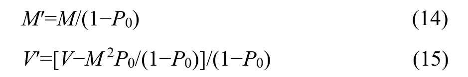
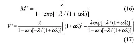
where M and V are the mean and variance of the complete distribution in Equation 2, respectively. By incorporating Equations 3, 4, and 10 into Equations 14 and 15, we obtain the mean and variance of the zerotruncated GP distribution:
1.3 Data analysis
From the count data in the community, I first denoted the observed SAD as follows: S1, species represented by one individual; S2, species by two individuals; …; Sr, species by r individuals; …, thus obtaining the frequency distribution of Sragainst r. I used the number of individuals per species, r, as a discrete random variable to fit the zero-truncated GP distribution.
I calculated the distribution parameters from a sample by using the maximum likelihood and valuetrying method in the software Mathematica 4 (Wolfram Research, Inc., 1999), i.e., finding precise estimates of the parameters such that the log likelihood function reaches a maximum (Yin, 2005; Yin et al., 2013),expressed as
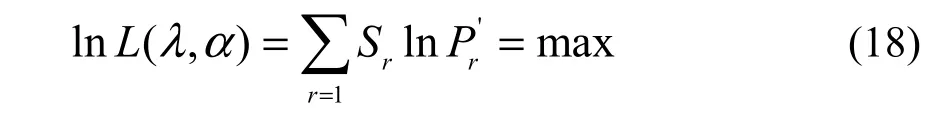
where lnL(α, λ) is the natural logarithm of likelihood function with relation to the two parameters α and λ; Sr, equivalent to the observed frequency of r individuals, is the observed number of species with r individuals; S1+S2+…+Sr+…=S, equivalent to the sample size, is the observed number of species in the forest community.
I tested the goodness of fit of the expected distribution to the observed distribution (i.e., SAD count data). Because of the nature of the dataset, the goodness-of-fit chi-square (χ2) test was applied(Glover et al., 2001). Finally, I compared the GP with the PLN in fitting the SADs through the Akaike information criterion (AIC) and the consistent AIC(CAIC), defined as (Akaike, 1973; Gurmu et al., 1996;Wang et al., 1997; Melkersson et al., 2000; Yin et al.,2013).
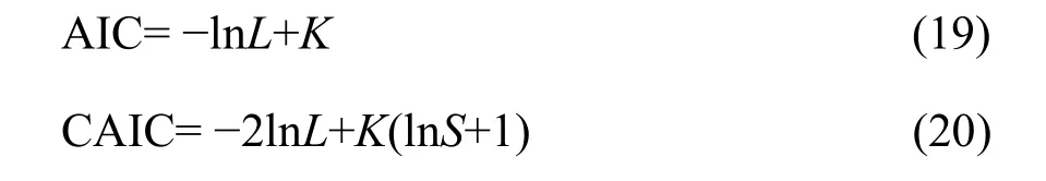
where lnL is the value of the log likelihood function, i.e., lnL(α, λ) in Equation 18; K the number of estimated parameters; and S the sample size (i.e., the observed total number of species in the study). A smaller AIC or CAIC value indicates a better fit to the model.
2 RESULTS
The investigation at the 1-ha permanent forest community plot in Dinghushan Biosphere Reserve,South China, showed that: (1) the tree layer had 3890 individuals that belonged to 69 species in 25400 m2subplots; (2) the shrub layer had 428 individuals of 39 species in 2525 m2quadrats; and (3) the herb layer had 151 individuals of 32 species in 25 1 m2subquadrats(Table 1).
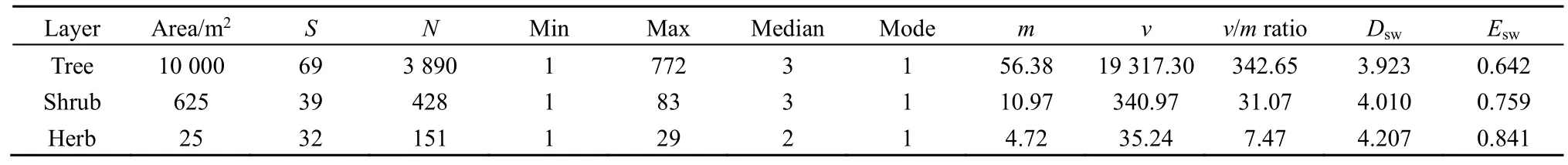
Table 1 The descriptive statistics of species abundances in the tree, shrub and herb layers of evergreen needle- and broad-leaved mixed forest community in Dinghushan Biosphere Reserve, South China
The Shannon-Wiener diversity indexes (Dsw’s) of the tree, shrub and herb layers in the forest community were 3.923, 4.010 and 4.207, respectively. The measures of equitability or evenness based on these indexes (Esw’s) were correspondingly 0.642, 0.759 and 0.841. Both diversity and evenness of species slightly increased from the tree, shrub to herb layer in the 1-ha community plot (Table 1).
The observed mean (m), variance (v) andv/mratio ofrdramatically decreased from the tree, shrub to herb layer. Moreover, all thev/mratios were much greater than one, suggesting obvious overdispersion, while the medians (=2-3) and modes (=1) for all the three layers were almost equal (Table 1).
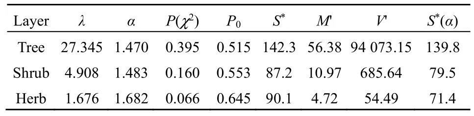
By plotting the number of speciesSrwithrindividual(s) againstr, the inverse J-shaped frequency distributions of the observed SADs in all three layers of the community was obtained (Figure 1). Since the observed variance of the random variablerwas much larger than the mean for each layer (Table 1) and there was an overdispersion in the SAD data, the zerotruncated GP distribution to describe this pattern is applied. The observed SADs in the three layers followed the zero-truncated GP distributions (chisquare test,P(χ2)>0.05; Figure 1 and Table 2).
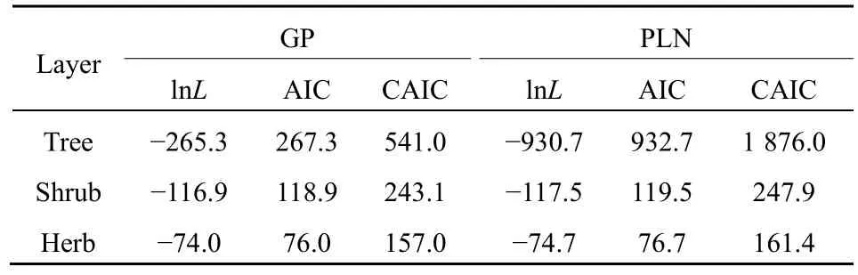
As to the GP distribution parameters, theλvalues significantly decreased from the tree, shrub, to herb layer in the community while theαvalues were close to one another although slightly increased (Table 2). In the expected zero-truncated distributions, the curve’s steepness was as follows: tree layer Figure 1 Comparisons of the zero-truncated generalized Poisson (GP) distributions fitted to the SAD data among the tree, shrub, and herb layers of evergreen needle- and broadleaved mixed forest community in Dinghushan Biosphere Reserve, South China Table 2 Fitting results of the zero-truncated generalized Poisson (GP)distributions to the species abundance distributions (SADs) in the tree,shrub, and herb layers of evergreen needle-and broad-leaved mixed forest community in Dinghushan Biosphere Reserve, South China In particular, of the two parameters of fitted GP distribution,αexhibited a more similar pattern to the diversity index thanλ(Tables 1 and 2). In other words,likeDsworEsw,αshowed little increase from tree, shrub to herb layer, i.e., the values ofαfor the three layers were very similar. Butλdecreased dramatically from tree, shrub to herb layer. it is also observed that theαvalue was nearly twice the evennessEswfor each layer,further suggesting that the parameterαcould describe the species diversity in the forest community. Comparisons between the observed and expected statistics for each layer (Tables 1 and 2) showed that the expected mean from the zero-truncated GP distribution was equal to the observed (i.e.,M′=m), indicating that the GP model fitted well to the SAD data; although the expected variance was much larger than the observed(i.e.,V′>v), they were in the same order of magnitude. Using the GP distribution well describing the SAD data, it is estimated the potential species richness, theS*and theS*(α) supposingλ→∞, in the three layers of whole community of given area. ForS*, the tree layer was dramatically the largest, followed by the herb and shrub layers that were very close to each other. This pattern was similar to the one forS*(α) except that the shrub layer was slightly greater than the herb layer in species richness for the latter.S*andS*(α) showed similar patterns to the observed total number of species,S, in the order of magnitude for three layers, althoughS*(slightly)>S*(α) (greatly)>Sfor each layer (Tables 1, 2). By comparing the GP and PLN distributions in the goodness of fit to the observed SADs in the forest community, it is observed that the former agreed with the data better than the latter in each of the three layers,as indicated by the smaller AIC or CAIC of the fitted GP than that of the fitted PLN for each layer (Table 3).There were different performances among three layers in AIC or CAIC: the values of GP were dramatically less than that of PLN for the tree layer, while the former were slightly less than the latter for the other two layers. Table 3 Comparisons of the goodness of fit between the generalized Poisson (GP) and Poisson lognormal (PLN) distributions in describing the species abundance distributions (SADs) of the tree, shrub, and herb layers of evergreen needle- and broad-leaved mixed forest community in Dinghushan Biosphere Reserve, South China The results showed that the discrete GP distribution could describe the SAD with the overdispersion of count data in the tree, shrub or herb layer of the evergreen needle- and broad-leaved mixed forest community in south subtropics of China. Peng (1996)found that: (1) the abundance of a species could affect the abundances of others in lower subtropical forests;and (2) the occurrence of a species could influence the invasion or establishment of subsequent species in succession. These are similar to the scenarios generating the GP distribution, as shown by Consul(1989) and Tuenter (2000). For another, overdispersion of each species, i.e., spatially clumped(Greig-Smith, 1983; Brown et al., 1995; He et al., 1997;Condit et al., 2000; Yin et al., 2005b), may lead to overdispersion of the collection (assemblage) of all species in a community. These are why the observed SADs followed the GP distribution. The GP distribution was better than the PLN in terms of the goodness of fit to the same SAD data collected in all the three layers of the forest, suggesting that the GP’s possibly broader applicability to the description of SADs with the over-dispersion in communities. Further, the AIC or CAIC of the GP was dramatically less than that of the PLN for the tree layer,while the former was slightly less than the latter for the shrub and herb layers. This may be due to the difference of sample sizes among the three layers. The more suitable GP distribution may have a wider application prospect than the PLN, especially in estimating the potential species richness in a community as well as on a local or regional scale and determining the species proportion for ecological restoration of degraded forests. For all the three layers of the forest community,the SAD curves were inverse J-shaped. The respective medians and modes were almost equal, and theαparameter values of the fitted zero-truncated GP distributions were close to one another. The similarities in the SADs among the three layers could be due to the homogeneity of macroenvironment at the same forest stand in the lower subtropical monsoon climate zone(Yin et al., 2005c). On the other hand, the SADs between the three layers also had some different properties, including the significantly decreasing means, variances, variance/mean ratios, andλparameter values of the GP distribution from the tree,shrub, to herb layer. This could be because of the heterogeneity of microenvironment in the layers of different height in the community. Based on fitted GP distribution to observed SAD,we can estimate the potential species richness, theS*and the S*(α) if λ→∞, in the whole community of given area. Based on the GP, S*values of the tree, shrub, and herb layer were 142, 87 and 90, while on the PLN,those were 211, 75, and 62 (Yin, 2005), respectively.Since the GP better fitted data than the PLN, the latter overestimated S*in the tree layer but underestimated those in the other two layers. S*(α) was slightly less than S*for each layer. This may be because that with the increase of total number of individuals, N, sampled in the community, the relatively large increase of the individuals of one or more common species results in the gradual disappearance of some rare species with ≤1 individual. For another, the methods above show that if λ→∞ and hence N*→∞, then S*converges to a limit,S*(α), suggesting that in a given area, the total number of individuals of all species can become very large but the total number of species tends to a given value, as indicated in the well-known species area relation (e.g.,May, 1975; Miller et al., 1989; Wei et al., 2014).Therefore, the above results can mirror the rationality of GP distribution to describe the SAD in a community. The two parameters α and λ controlled the zerotruncated GP distribution’s scale and shape. The distribution was hump-shaped (unimodal) when 0≤α≤0.291 and λ≥2.01; otherwise, it was inverse J-shaped (or hollow, hyperbolic). In this study, for all the layers of the community, α>0.291; therefore, the distribution curves were all inverse J-shaped.Furthermore, when α≥1.1 and λ≥1.2, the larger α or the smaller λ, the smaller the curve’s slope rate (<0) at any point of r, suggesting the greater steepness of the inverse J-shaped curve. This may explain why the distribution curve was steepest for the herb layer,followed by the shrub and tree layer (Figure 1). A steeper SAD curve implies more rare species(particularly singletons) and thus fewer common species in a community, and consequently suggests a lower steepness of rank abundance curve (Yin, 2005;Yin et al., 2005c). It also indicates a higher Shannon-Wiener index of diversity (Dsw) or evenness (Esw),which is one of the most common measures of diversity(Krebs, 1978, 2001; Yin, 1998; Xian et al., 2014; Yin et al., 2014; Chen et al., 2020; Lv et al., 2020; Li et al.,2021; Zhong et al., 2021). This is the case in the study:herb layer>shrub layer > tree layer, for the steepness of SAD (Figure 1) as well as for the Dswand Esw(Table 1;Yin, 2005). As mentioned above, species diversity was positively related to α but negatively correlated with λ.As shown in Equation 10 and Table 2, P0increased with decreasing λ and increasing α, suggesting that species diversity was positively related to the probability of species not collected in a sample. Further, the SADs were often more informative than some species diversity indices (Novotny, 1993). Of the two GP parameters, α could better reflect the species diversity than λ because: (1) α indicated the variation and overdispersion of the SAD (the more the variation, the higher the diversity), while λ represented the mean of the SAD, and thus α was independent of, while λ was dependent of, sample size (i.e. the observed total number of species S, or sampling area); and (2) α showed more similar trend to the diversity index (Dswor Esw) than λ for each case. Consequently, α can be a good measurement of species diversity in the community. A discrete GP distribution with two parameters α and λ can well describe the SADs in all the three major layers (tree, shrub, and herb) of an evergreen needleand broad-leaved mixed forest. it is also found that, (1)the SADs follow the zero-truncated GP with significantly decreasing λ and slightly increasing α from the tree, shrub, to herb layer and are inverse J-shaped due to the interplay between α and λ. (2) the GP distribution shows a better goodness-of-fit to the SAD data than the PLN distribution, which discretizes the commonly-used continuous lognormal with the Poisson. The GP is suitable for the discrete SAD data with overdispersion and may have broader application than the PLN, and the parameter α is a good measure of species diversity in a biotic community. By fitting the GP distribution to observed SAD, one can better predict the potential species richness (S*) than PLN in a community as well as on a local or regional scale. ACKNOWLEDGEMENTS:Thanks to Dr. Prof.Qinfeng Guo within Eastern Forest Environmental Threat Assessment Center, USDA Forest Service, USA for the help in English. I thank: Shao-Lin Peng within School of Life Sciences, Sun Yat-Sen University (Zhongshan University); Hai Ren, Qian-Mei Zhang, Zhong-Liang Huang and Guo-Yi Zhou within South China Botanical Garden (SCBG), the Chinese Academy of Sciences; and many others for their help in field work and manuscript revision. I also thank the Dinghushan Forest Ecosystem Research Station of SCBG in Dinghushan Biosphere Reserve, Guangdong, China. This study was supported mainly by the grant from Provincial Major Project of Education Department of Guangdong Province, China(No. 2016KZDXM002). The other funding projects included: the Guangdong Nature Science Foundation (No.06300348), Wang Kuancheng Research Prize Project of Chinese Academy of Sciences (No. 2006-65), the Forestry Science and Technology Research Planning of Guangdong Province (No. 2003-2), the National Natural Science Foundation of China (Nos. 30270282 and 30200035), the Guangdong Spark Program (2KB 05901N), the National Science and Technology Supporting Plan of China (No. 2012BAD22B05), and the ITTO Project (No. PD 294/04 F).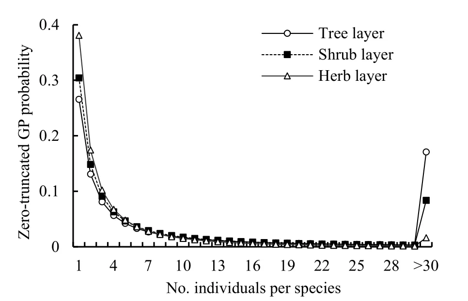
3 DISCUSSION
3.1 Relation of GP distribution and over-dispersed SAD
3.2 Comparison of GP and PLN distribution
3.3 Difference of GP distribution parameters among layers
3.4 Potential species richness estimated by GP distribution
3.5 GP distribution parameters and SAD curve shape
3.6 GP distribution parameters and species diversity
4 CONCLUSIONS