Identification of heavy metal-contaminated Tegillarca granosa using laser-induced breakdown spectroscopy and linear regression for classification

Zhonghao XIE (謝忠好), Liuwei MENG (孟留偉), Xi’an FENG (馮西安),5,Xiaojing CHEN (陳孝敬), Xi CHEN (陳熙), Leiming YUAN (袁雷鳴),Wen SHI (石文), Guangzao HUANG (黃光造) and Ming YI (衣銘)

1 School of Marine Science and Technology, Northwestern Polytechnical University, Xi’an 710072,People’s Republic of China

2 College of Physical and Electronic Information Engineering, Wenzhou University, Wenzhou 325035,People’s Republic of China

3 Research and Development Department, Hangzhou Goodhere Biotechnology Co., Ltd, Hangzhou 311100, People’s Republic of China

4 Research and Development Department, Hangzhou Weizan Technology Co., Ltd, Hangzhou 311100,People’s Republic of China

5 Authors to whom any correspondence should be addressed.

Abstract Tegillarca granosa (T. granosa) is susceptible to heavy metals, which may pose a threat to consumer health. Thus, healthy and polluted T. granosa should be distinguished quickly. This study aimed to rapidly identify heavy metal pollution by using laser-induced breakdown spectroscopy (LIBS) coupled with linear regression classification (LRC). Five types of T.granosa were studied, namely, Cd-, Zn-, Pb-contaminated, mixed contaminated, and control samples. Threshold method was applied to extract the significant variables from LIBS spectra.Then, LRC was used to classify the different types of T. granosa. Other classification models and feature selection methods were used for comparison.LRC was the best model,achieving an accuracy of 90.67%. Results indicated that LIBS combined with LRC is effective and feasible for T. granosa heavy metal detection.

Keywords: shellfish, laser-induced breakdown spectrometry, heavy metal, linear regression classification

1. Introduction

Tegillarca granosa(T. granosa), which is also called blood cockle because of the red liquid inside its soft tissues, has become a preferred aquatic product among consumers because of its rich nutrients [1]. Various toxic heavy metals are discharged into rivers and oceans as a result of industrial development.T. granosais vulnerable to heavy metal absorption and contamination due to low activity and filterfeeding.Moreover,enriched heavy metal elements transfer to the food chain and accumulate in the human body after people eat contaminatedT. granosa, which may result in the risk of chronic poisoning [2, 3]. Thus, whetherT. granosais contaminated by heavy metals should be determined.

Many methods are used to detect heavy metal ions,such as flame atomic absorption spectrometry, graphite furnaceatomic absorption spectrometry, atomic fluorescence spectrometry, infrared spectroscopy, and inductively coupled plasma mass spectrometry [4-10]. Although some of these methods have high sensitivity and accuracy, they are either high cost, time-consuming or need to be conducted by experienced technicians. As a rapid analytical technique,laser-induced breakdown spectroscopy (LIBS) requires minimal or no sample preparation, suitable for fast and free reagents, thereby making it a promising rapid detection method[11].In LIBS,the sample is ablated by using a highly energetic laser pulse and a high-temperature plasma is produced. Shortly afterward, light is emitted during the cooling of the plasma, and the spectra are recorded with a spectrometer. The emission lines corresponding to the special element are collected and analyzed [12]. In this way, LIBS provides several elemental data of a sample in a single measurement. LIBS has been successfully applied to analyze and detect elements in multiple fields, such as geological analysis [13, 14], food safety [15-17], environmental monitoring [18], and space exploration [19, 20].

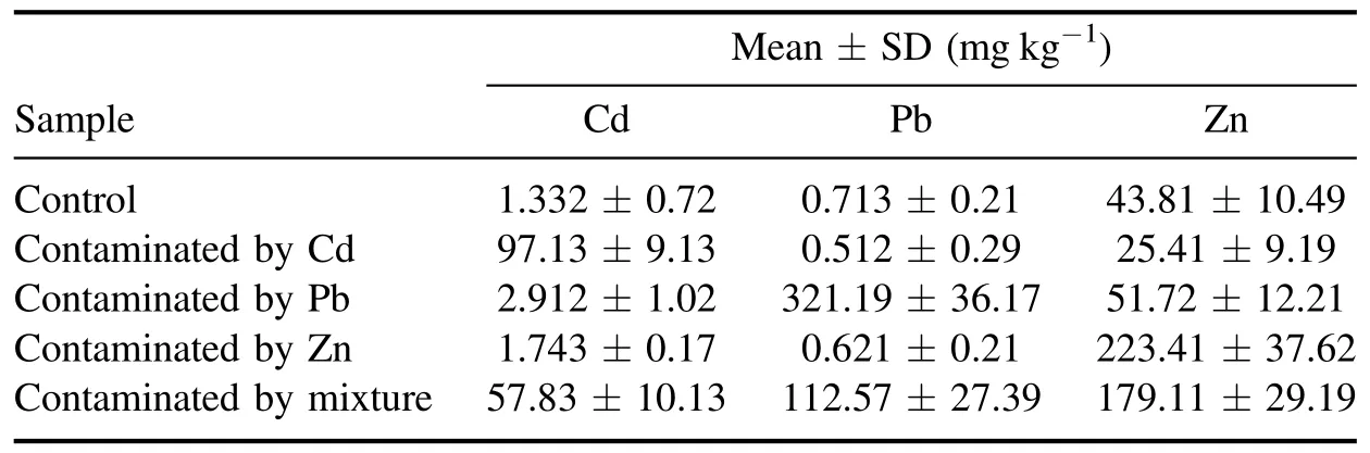
Table 1.The heavy metal content statistical values of 150 T. granosa samples.

In general,LIBS data contain thousands of variables and can be analyzed rapidly and accurately by coupling machine learning and statistical techniques [21-23], such as partial least squares (PLS) [24-26], support vector machine (SVM)[27,28],and k-nearest neighbor(kNN)with LIBS[29].These methods can achieve the goal for the qualitative and quantitative analysis of LIBS data. However, these algorithms are all parameterized, and sometimes training the model to achieve a satisfactory result is time-consuming. In addition,due to the redundancy, complexity, and instability of the original LIBS data [11], these multivariate algorithms may not perform well when full variables are used to establish the classification model. To overcome this obstacle, various simple but efficient methods, including threshold method(TM) and linear regression classification (LRC), have been developed to distinguish different kinds of samples.LRC is a nonparametric and powerful method and does not require training.The main steps of this approach are as follows:first,we use TM as a feature selection method to remove a large amount of irrelevant information from the LIBS spectra,then,on the basis of the remaining feature data, we use LRC as a classifier.

In this research, five groups ofT. granosa, namely,uncontaminated control samples; samples contaminated with cadmium (Cd), zinc (Zn), and lead (Pb); and samples contaminated with three heavy metal mixtures, were used to assess the efficacy of the proposed method. Other classification methods, such as PLS-discriminant analysis (PLS-DA)[30], SVM [31], kNN, linear discriminant analysis (LDA)[32], and feature selection methods, such as variable importance of projection(VIP)and random frog(RF),were adopted for comparison. The specific objectives are (1) to obtain the LIBS data of contaminated and uncontaminatedT. granosasamples,(2)extract the useful feature from original LIBS data for the classification model,and(3)evaluate the performance of the proposed LRC method.

2. Materials and methods

2.1. Sample preparation

T. granosasamples, which were provided by Zhejiang Mariculture Research Institute (Wenzhou, China), were acclimatized to laboratory conditions for 10 d in plastic pools. The studiedT. granosasamples were randomly divided into five groups, with 30 samples for each experimental group. The samples in Pb, Cd, and Zn groups were exposed to water dissolved with highly concentrated PbCH3COO · 3H2O(1.833 mg l-1), CdCl2(1.634 mg l-1), and ZnSO4· 7H2O(4.424 mg l-1). The mixture group was exposed to a mixture with equal amounts of the above three chemicals.The control group was raised in seawater and used as the blank control group.The seawater in the containers had a pH of 8.45 ± 0.4,a dissolved oxygen content of ＞6 mg l-1, a temperature of 24.8 ± 5.6 °C,and a salinity level of 21%.For each 24 h,all the containers were refilled with new seawater and dosed with the corresponding metal toxicant. At the end of the 10 d rearing period,the samples were removed from plastic bowls and placed in a ?4 °C refrigerator.Then,these samples were freeze-dried, ground into powder, and compressed for subsequent spectral measurement.

The concentration values of Cd, Zn and Pb were measured by a NexION 300X ICP-MS (NexION 300X, Perkin Elmer, Inc., U.S.). The statistical values of the three heavy metal contents (Cd, Zn, and Pb) of the samples are listed in table 1.

2.2. LIBS spectra collection

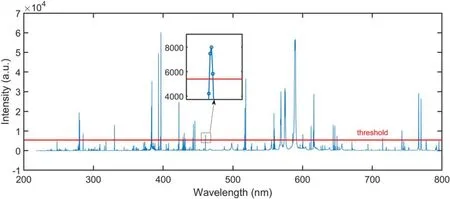
Figure 1.Feature selection using threshold TM (threshold = 5400).

The experimental measurement platform used in this study consisted of a Nd:YAG laser (Litron Nano SG 150-10, Litron Lasers,Warwickshire,England),a triple prism,a plano-convex lens (f= 100 mm), an optical fiber system, a spectrometer(LTB Aryelle 150, Berlin, Germany), and a charge-coupled device (CCD). Nd:YAG was used as the laser source with a wavelength of 1064 nm,a pulse duration of 6 ns,and an energy of 150 mJ.The laser beam was reflected by the triple prism and focused onto the sample by the lens.A beam splitter was used to split a small fraction of energy (about 10%) for monitoring the pulse energy. To reduce atmospheric interference, the distance between the lens and the test sample was optimized.The light from laser-induced plasma was collected by a fiber optic system and fed into the spectrometer equipped with an optical chopper (with a time resolution of 0.1 μs). The spectrometer was synchronized with the laser, and its spectral resolving power was 6000. The CCD was utilized for the spectra acquisition and its gate width was 30 μs. Each sample was measured five times at different spots on the translational stage,and each spectrum corresponded to an average of these measurements.

In addition, to improve the detection accuracy of contamination at certain local areas, the spot diameter on the surface of the test sample was adjusted to 500 μm.

2.3. Feature selection

Feature selection obtain a subset of relevant features from original data. LIBS data collected in this study have more than 30 000 variables, with most of them being low-intensity and uninformative variables. Appropriate feature selection helps reduce training times, defy the curse of dimensionality,and improve prediction performance. In this study, TM was adopted to extract the features from LIBS data. For comparison, other feature selection methods, such as RF and VIP[33], were introduced.

2.3.1. Threshold method. TM is a simple feature selection method. It retains all the variables with a value greater than the given threshold (T). Considering that the peak of LIBS data has the most significant and important information, a threshold was set to extract the variables whose intensity was greater thanT. In this study,Twas applied in the average spectrum of the calibration set to obtain the global feature for all samples. As shown in figure 1, the curve represented the average spectrum, and most of the variables were discarded when the threshold was about 5000. The remaining variables formed the feature set for model construction. To determine the optimal threshold, a range of thresholds were evaluated.According to the range of intensity in the spectra,we searched an appropriate threshold from ?300 to 24 000 (with a stride of 300). The corresponding feature set of each threshold was verified by LRC. The threshold whose corresponding feature set has the best accuracy was chosen as the optimal threshold.

2.3.2. Variable importance in projection. VIP variable selection method is widely used in feature selection and was first proposed by Wold in 1993 [34]. The VIP scores obtained in the PLS analysis reflect the influence of each variable on the model. The variables with high VIP scores contribute to variance explanation of the response. The equation for calculating VIP scores for thejth variable is provided in the literature [35]. The average of squared VIP scores is equal to one. Thus, the greater-than-one rule is always used as a criterion for variable selection.In this study,considering that no statistically justified standard exists for VIP, we searched for the best cut-off in a grid of values ranging from 0.5 to the maximum value of VIP scores,instead of assigning a fixed value.

2.3.3. Random frog. RF is named because the process simulates the foraging behavior of a group of frogs. The details of this process can be found in the literature [36]. A selection probability of each variable is obtained at the end of this approach.The probabilities ranging from 0 to 1 provide a useful measurement to select the useful variables. Similar to VIP scores,the variables with high probability are more likely to be selected into the final model. To obtain the optimal feature data,the criterion for probability ranges from 0.1 to 1.

2.4. Classification model

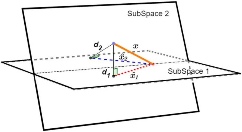
Figure 2. Unlabeled sample x is projected into two subspaces.Distance (d) reflects the similarity between x and the subspace.

2.4.1.Linear regression for classification. The LRC algorithm is a simple, powerful general process to determine the similarities between the given samples and the subspace [37].LRC can be categorized as a nearest subspace approach.GivenNsubspaces,unlabeled sample x is projected on each subspace spanned by the samples with the same category via the least square method [38]. The Euclidean distance between the projection and x is used to measure the degree of membership between the sample and subspace.In general,x is considered to belong to the subspace with the minimum Euclidean distance.The LRC process is described in figure 2.

Some formulas are shown to explain the process of LRC.Assuming that every spectral sample data is a 1 ×pvector,we arrange the givenntraining samples from theith class as columns of a matrix Xi,Xi= [xi,1,xi,2,…,xi,n] ∈ IRp×n,where xi,jdenotes thejth sample from theith class, xi,j∈ IRp×1.

Given sufficient training samples for each class, any test sample x from theith class lies approximately in the linear span of these training samples.

where ai,jdenotes the regression coefficient ofdenotes the projection ofxon the subspace ofith class Xi,ai= [ai,1,…, ai,n]T, ai∈ IRn×1.

Obtaining representation aisolves the inverse problem as follows:

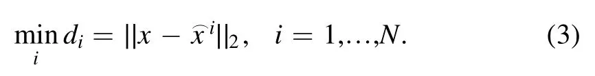
The distance dibetweenand x presents the membership of the sample and theith class. The object with the minimum distance is the best candidate, which can be formally expressed as follows:

2.4.2. Other classification models. PLS regression uses projection to relate response y to a set of predictor variable X and is extensively used in various domains.PLS-DA can be regarded as a special PLS regression[30],where response y is a discrete variable rather than a continuous variable. The essential issue in building a PLS model is how to determine the number of latent variables (nLvs). An inappropriate number of latent variables can lead to overfitting or underfitting problems.In this work,nLvsranged from 7 to 13.

SVM is one of the most prominent classification models[31].By constructing a hyperplane or a set of hyperplanes in a high-dimensional space, SVM effectively separates the different classes in training data. SVM is originally developed for binary classification and can be applied in multi-classification with strategies,such as one-against-one and one-against-all.As well known,the parametersCand γ are important in designing a powerful SVM model. In this study, the values ofCand γ vary asC= {2-5,2-3…,215}and γ = {2-15,2-13…,21}.A grid search was utilized to get the optimal parameters.

kNN is a simple classification method [29]. Given an unknown sample x,knearest samples of x are obtained from the calibration set. Commonly, the Euclidean distance is utilized as the distance metric. Then, the label of x is determined through the voting of theseksamples. Unlike other classification models such as SVM, kNN requires no real training process before prediction. For kNN, deciding suitable initialkvalue is essential factork, which can greatly affect the performance of kNN. In this study, the value ofkwas picked fromK= {3, 5, 7, 9, 11}.

LDA is a classification method which has been successfully applied in many classification problems [32].Similar to principal component analysis(PCA),LDA is often used as a dimension reduction method in statistics and machine learning. The aim of LDA is not to find a linear combination of features that presents the largest variance of X as PCA does but to find several components that are considered to be the most helpful for classification.Generally,the number of components is limited and lower than the number of classes. In this study, the number of components was the only parameter for LDA and ranged from 1 to 4.

2.5. Overview

The main process of our classification method is shown in figure 3. It includes sample preparation, spectra collection,spectra analysis, feature selection, and model validation. In conducting spectrum analysis, PCA was used for exploratory analysis [39]. The feature set was obtained by TM, which selected the most useful variables from the original data.Each feature set extracted under different thresholds was evaluated,and the feature set with the highest accuracy was chosen as the optimal feature set. VIP and RF were adopted for comparison.The feature set was randomly divided into calibration and testing sets; the calibration set was used to train the classification models, and the testing set was used to verify their performance. Among all classification models listed in figure 3,it is worth noting that LRC is the only model that is parameter-free and does not need any training.

2.6. Algorithm implementation

All model algorithms were performed in MATLAB 2010b(The Math Works, Natick, MA). The performance of these models was evaluated in terms of their accuracy, which was acquired by five-fold cross-validation [40]. To optimize the parameters of each model, the same cross-validation was utilized.

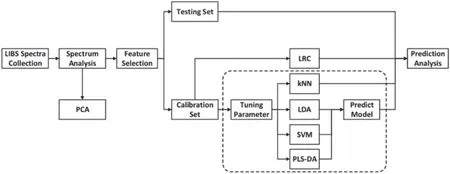
Figure 3.Main process of LIBS coupled with classification models.

3. Results and discussion

3.1. Analysis of LIBS spectra

In this study, the spectral data of five groups ofT. granosasamples were obtained. Each spectral data contained 30 267 variables. As shown in figure 4, the typical spectrum ofT.granosacontained dozens of characteristic peaks.The atomic and ionic lines of Al, C, Ca, Cd, Fe, K, Na, Mg, Pb, Si, Sr,and Zn spread over the wavelength range (200-800 nm).There are emission lines with high intensity, such as Ca I(422.7 nm), Ca II (393.3 nm, 396.8 nm), Na I (588.9 nm,589.5 nm), Mg I (285.2 nm, 517.3 nm, 518.4 nm), Mg II(279.5 nm, 280.3 nm), and K I (766 nm, 770 nm). Less prominent emission lines, like C I (247.8 nm), Zn I(330.3 nm),Sr I(460.7 nm),Si I(288.2 nm),and Fe I(438.4 nm, 440.5 nm), can also be found in the spectra. Though some characteristic peaks in the LIBS spectra are remarkable,like Zn I (330.3 nm), many peaks of target heavy metals are seriously interfered. Due to various reasons, such as matrix effect, self-absorption, other background interference, there are not enough significant peaks of target heavy metal elements (Pb, Zn, and Cd) to perform the classification task effectively. Therefore, chemometric methods need to be introduced for further analysis.

As an exploratory method,PCA was adopted to draw the distribution scatter plot (PC1 and PC2) of the spectra. As shown in figure 5, the two primary components explained only 54.13% of the data variance, indicating that the composition of LIBS data was complicated. Moreover, these samples were very similar to each other. In this study,separating the samples was difficult by ordinary classification approaches, thus requiring a robust and sensitive method.

3.2. Classification results based on full spectra

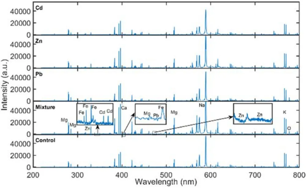
Figure 4.Representative spectra of the analyzed T.granosa:Cd,Zn,Pb, mixture and control.

Taking one typical Cd-contaminated sample as an example,we calculated its projection on the subspaces of five groups by using LRC.To simplify the illustration,only the first three projections(Cd,Zn,Pb)are shown in figure 6.Low-intensity variables were seriously disturbed by noises, which made them less informative. Thus, they should be removed before modeling. Besides, as we can see from figure 6, though the projection of the sample on each group had a small difference,the projection on the Cd group was the closest to the original sample. Taking advantage of this, LRC can achieve high sensitivity.

To explain LRC in detail, three samples were randomly removed from the Cd group and projected into the space of the five groups. The Euclidean distance between the samples and their projections is plotted in figure 7.Sample 1 was treated as a Cd-contaminated sample because its absolute distance from the Cd group was the closest. In addition, the distances between the samples from five different groups conformed to a similar pattern. For the Cd group, the mixture group was the closest and the Zn group was the farthest in most cases.In the case of misclassification, the samples from the Cd group were more likely to be treated as Mixture than Zn.

Using the full spectral data, the accuracy of LRC reached 77.3%, whereas other classification models, including kNN,LDA, PLS-DA, and SVM, did not perform as well as LRC,having accuracies of 27.33%, 37.3%, 49.3%, and 37.3%,respectively. Despite the high similarities within the data samples, LRC performed better than other classification models.

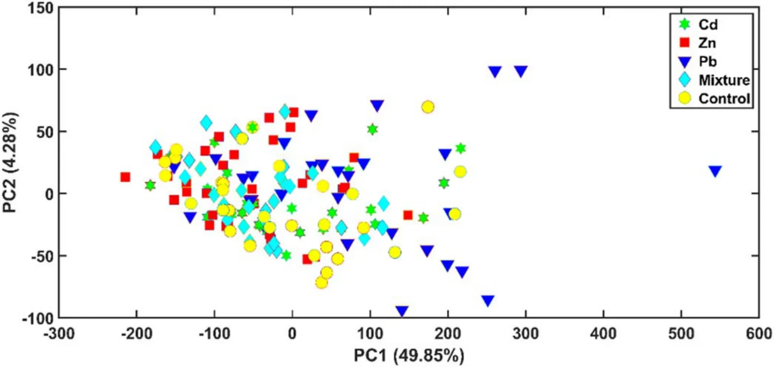
Figure 5. PC1 and PC2 scores to present the similarities between the LIBS spectra of different T. granosa.

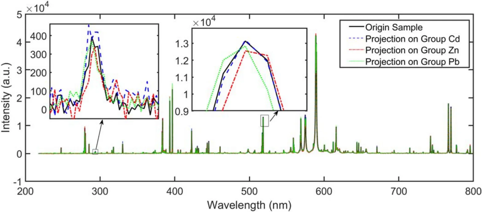
Figure 6.Typical spectra of the Cd group and its projections on three subspaces (Cd, Zn, Pb).

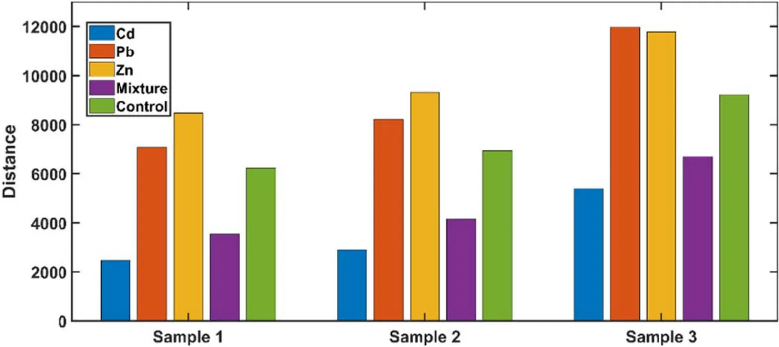
Figure 7.Three samples were randomly selected from the Cd group and their distances from each subspace of the five groups.

3.3. Classification results based on feature variables

Many irrelevant and redundant variables were present in the spectral data,thereby potentially increasing the complexity of the model and lowering the performance.Hence,these useless variables should be removed before modeling. To extract the feature, TM was adopted and a range of thresholds, from?300 to 24 000, were evaluated. A large threshold corresponded to a few selected variables. As shown in figure 8,the number of selected variables dropped dramatically in the beginning. Then, the rate of descent slowed down after the threshold exceeded 1000 and the number of selected variables eventually reached around 47.

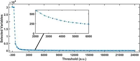
Figure 8. Number of selected variables versus the threshold value.

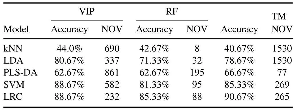
Table 2.Comparative results of VIP,RF,and TM combined with kNN,LDA,PLS-DA,SVM,and LRC.Accuracy values greater than 85%are presented in bold.

To compare TM with VIP and RF, we used LRC and other models to verify all the feature sets obtained by these feature selection methods. The result of each combination is shown in table 2,with its best accuracy and the corresponding number of optimal variables (NOVs). Among the three feature selection methods, the performance of RF was relatively poor, but its NOVs were less than that of the other two methods.In most cases, TM required the most NOVs, but its overall result was better than that of VIP and RF.To measure the importance of each variable,both VIP and RF rely on the result of PLS, while determining the appropriate latent variables for PLS is not always easy.Unlike VIP and RF,TM did not need to measure the importance of each variable to obtain the optimal feature data and was thus easy to conduct.Together all, TM performed better than VIP and RF in this study.

To obtain the optimal feature set, we used LRC to evaluate all feature sets extracted by various thresholds. For comparison, other classification models were performed on these feature sets.All models with parameters were optimized to achieve optimal results. As shown in figure 9, initially, all algorithms used the full spectra when the threshold was-300.At this time, the accuracy of LRC was significantly higher than that of other algorithms, thereby showing that the LRC model had better robustness than other models. As the threshold increased, all models obtain incremental performance improvements due to a large number of unrelated variables being discarded. SVM had the sharpest increase,from 37.3% to over 80.0%. When the threshold was around 5400, LRC presented the best result with an accuracy of 90.67%,and the number of selected variables dropped to 265,providing a cut rate of 99.1%. The accuracy curve of each model dropped slowly after it approached its maximum accuracy value due to the decrease of useful information. However, the accuracy of all classifications was not greatly affected although the threshold reached 24 000 and fewer than 50 variables remained in the feature data. These results showed that the characteristic peaks with high intensity played a decisive role in the classification.

3.4. Discussion

As mentioned in section 3.2, among the five groups of samples, the Mixture group was the closest to the Cd group,followed by the Control group. As shown in the confusion matrix in table 3, six samples from the Cd group were misclassified; four samples were misclassified as Mixture, and two samples were misclassified as Control. Similarly, two misclassifications were observed in the Mixture group, being misclassified as the Cd group.

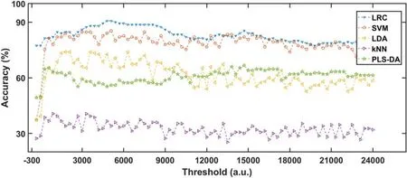
Figure 9. Accuracies of LRC, SVM, LDA, kNN, and PLS-DA versus the threshold.

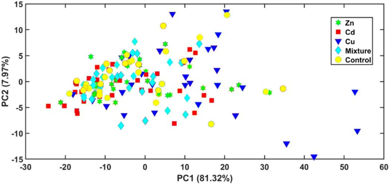
Figure 10.PCA plot based on the feature data extracted by using TM (T = 5400).

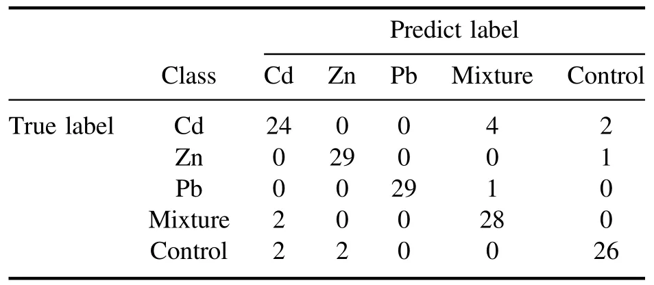
Table 3.Confusion matrix of LRC combined with TM (T = 5400).

The above results show that LRC was more effective than the other classification models. Although most of the classification models improved after feature selection, their results were still poorer than those of LRC model. In particular, the accuracy of kNN was always below 50%, while LRC performed far better than kNN.To explore this problem,PCA was applied in the feature data extracted underT= 5400,where LRC presented the best accuracy.As shown in figure 10, PC1 and PC2 interpreted about 90% of the variance of this data because a large number of unrelated variables were removed.However, the samples were difficult to be distinguished because of their high similarity.For kNN,its decision depends onkclosest training samples of the test sample.Hence, kNN is prone to be ineffective when the data samples cannot be clustered properly, as shown in figure 10.Particularly, data in a high dimensional space tends to be sparser than in lower dimensions. In this case, for most data points, their distances tend to be close. Thus, the Euclidean distance of data samples, regularly used by kNN, is not informative. Instead of finding the nearest neighbors, the aim of LRC is to find the nearest subspaces of the test samples.In this case, all training samples are taken into account for the classification, which makes LRC quite robust in the discrimination task.That is why LRC and its variants have wide applications in machine learning and face recognition.

Until now, there is one thing left to be clarified, that is,which emission lines were selected after feature selection?For example,when LRC achieved its optimal accuracy, most of the selected lines belong to atomic like Ca II (393.3 nm,396.8 nm), Na I (588.9 nm, 589.5 nm) and Mg I (285.2 nm,517.3 nm, 518.4 nm) due to their high intensity. Affected by the heavy metal, the emission lines of these atomic have strong relevance with the concentration of target heavy metal.One possible reason for the relevance is that biological tissues of the contaminated samples are stressed by heavy metals to generate various metal oxides. Then, the different matrix effects lead to different spectral signals. Hence, they are also important for classification. Part of the selected lines belong to target heavy metal (Zn, Cd, Pb) like Zn I (330.3 nm) and other atomic with less prominent intensity.Unfortunately,the quantity of the lines from target heavy metal was inadequate for classification. Thus, we used all selected lines to do the discrimination mission and obtained a satisfying result.

As a powerful and simple classifier, LRC was successfully applied in the analysis of LIBS data.Still,there is room for improvement. TM is simple, worked well with the LRC model, and did not need to evaluate the contribution of each variable to the classification results, which may, on the other hand, introduce unrelative variables and affect the model’s performance.As a powerful tool and popular idea,sparsity is widely used in regression and classification,and it can surely be combined with LRC to improve its performance. In the future, we will work in this direction to improve the capabilities of LRC.

4. Conclusion

In this study,LIBS was used to detect the heavy metals inT.granosa. LIBS data are most commonly difficult to analyze due to high complexity and dimensionality,which resulted in the poor performance of classification models. To solve this problem,TM and LRC were adopted.The results showed that LRC combined with TM is a simple and powerful classification strategy, reaching an accuracy of 90.6%. Among the three feature selection methods,TM is more suitable for LRC than VIP and RF.Moreover,LRC performed better than other approaches, such as kNN and PLS-DA. These results demonstrate the effectiveness of the proposed LRC and TM framework, thereby providing a new analytical method for LIBS data.

Acknowledgments

This research was funded by National Natural Science Foundation of China (Nos. 31571920, 61671378).