Numerical and experimental study of continuous and discontinuous turbidity currents on a flat slope *

Zhong-luan Yan （嚴(yán)忠鑾）, Rui-dong An （安瑞冬）, Jia Li （李嘉）, Yun Deng （鄧云）, Yong Li （李永）,Ya-ya Xu （徐亞亞）

1. State Key Laboratory of Hydraulics and Mountain River Engineering, Sichuan University, Chengdu 610065,China

2. Postdoctoral Research Station, China Three Gorges Corporation, Beijing 100038, China

3. Water Resource and Hydropower Investigation, Design and Research Institute Co. Ltd. of Gansu, Lanzhou 730099 , China

Abstract: When the sediment and the dissolved matter laden in the river meet a clear water in reservoirs, the turbid water will plunge and spread into the clear water, forming the turbidity current and influencing the water quality and the life of the reservoir. Due to the unsteady nature of the flood, the turbidity current is unsteady. In the present study, we use the MIKE 3 computational fluid dynamics code to simulate continuous and discontinuous turbidity currents on a flat slope. With the model used by us, the turbulence is divided into two parts: the horizontal turbulence and the vertical turbulence, which are separately modeled by the Smagorinsky model and our model to capture the anisotropic turbulence. In this model, the sediment settling and deposition are considered. The simulation results concerning the flume water surface level, the front velocity and sediment concentration profiles are found consistent with the experimental data, particularly, for the sediment concentration profiles with an absolute mean error of 0.026 kg/m3 and the root mean square error of 0.046 kg/m3. This finding suggests that this model can be used to well predict the turbidity current on the flat slope.

Key words: Turbidity current, discontinuity, numerical model, turbulence, Smagorinsky model

Introduction

The flows induced by density differences between the inflow and the ambient flow can be classified into the density current, the gravity current and the turbidity current. In the nature, many phenomena are related with these kinds of flows: (1) In the meteorological field, the thunderstorm sea breeze fronts and the sandstorms are the results of the density difference induced by the temperature differences or the sand-laden between the spreading cold front and the warmer surrounding air[1]. (2) In the oceanographic field, the lava head for the sea is resulted from the turbidity current, which flows into the sea and moves onto the seabed[2]. (3) In the hydraulic engineering, the density currents are resulted from the differences in salinity, sediment or temperature. They are very important for the management of the sediment deposition and the water quality in reservoirs,lakes and rivers[3]. (4) Other forms of density currents include the discharge of hot water into cold water, the avalanche of snow[4], and the spillage of oil. When a river flows into a reservoir or lake, three configurations of density currents may occur, reflecting a slight difference in the salinity, the sediment concentration or the temperature. If the river water is lighter than the surface water, then the current flows similar to an overflow. However, if the river water is denser than the ambient water, then it will plunge under the ambient water and move similar to an underflow.When the river water has a density similar to that of the ambient water at a certain depth, it will plunge the ambient water and flow similar to an underflow in the early stages, and subsequently separate from the bed and propagate horizontally at a certain depth similar to an interflow. Zeng et al.[5], Chung et al.[6]and An and Julien[7]reported such currents. The turbidity current resulting from the sediment-laden inflow carries the suspended or dissolved sediment, which greatly influences the distribution of the sediment deposition and the pollutant matter in reservoirs or lakes. Hence,the turbidity current is significantly relevant to the water quality and the life of reservoirs.

The turbidity currents were observed in situ,including the Lake Mead, the reservoir of Tennessee Valley, and the Wellington reservoir. Many studies examined the turbidity currents. Ellison and Turner[8]studied the gravity currents spreading on a slope into a tank, showing that the mean fluid velocity has no relationship with the downslope distance. Janocko et al.[9], Motanated and Tice[10]have investigated the horizontal and vertical distributions of velocity and sediment concentration and the relationships among the front velocity, current thickness, water depth and inflow conditions. Dai[11]also conducted similar experiments and observed that the slope of the bottom qualitatively influences the flow pattern of the gravity current.

The structure and the behavior of the turbidity currents were numerically examined in several studies.In reality, the turbidity currents are 2-D or 3-D in nature. Hence, the detailed simulations of the turbidity current require 2-D or 3D models. Using the -kε turbulence model, the behavior of the various variables of the turbidity currents have been investigated[12]. An[13]applied the multiphase model to study the characteristics of the turbidity current plunging.Guo et al.[14]employed a 2-D multiphase model to simulate the flow structure and the density distribution in the gravity current. Imran et al.[15]employed a 3-D model to simulate the density current in a straight channel and verif i ed his model by comparison with the 2-D turbidity current experimental data.Firoozabadi et al.[16]simulated the 3-D motion of the dense underflows in a straight channel using the lower Reynolds number -kε model. The results of these simulations are consistent with the results of previous experiments. The 2-D or 3-D large eddy simulation(LES) and the direct numerical simulation were also been conducted to investigate the density currents generated from instantaneous sources and to identify the density differences in salinity[17-19]. In addition, the DNS and the LES are limited to the low Reynolds numbers, due to related high computational costs.

Although these experimental and numerical investigations revealed the flow characteristics of the turbidity currents under various conditions, the discontinuity of the turbidity currents has not been taken into considerations, especially on a flat slope.Because the floods can trigger the intrusion of highly turbid waters into reservoirs with a large amount of suspended sediment, the floods experience unsteady processes, making the turbidity current unsteady and discontinuous. In the present study, the computational fluid dynamics code Mike 3 based on the Navier-Stokes equations and the scalar transport equation is employed to simulate the flow and the sediment transport of the turbidity currents on a flat slope. The horizontal eddies are simulated using the Smagorinsky model, and the vertical eddies are simulated using themodel, with consideration of the effects of buoyancy on the turbulence. In this model, the particle settling and the sediment deposition are also considered, and the model is well validated against the experimental data.

1. Experimental setup

A laboratory flume is used to study the density current. The flume is shown schematically in Fig. 1.This flume is made of tempering glass, braced with a steel frame and is approximately 20 m long, 0.40 m wide, and 1 m deep, and the slope of the flume can be adjusted from 0% to 4%. In the present study, experiments are conducted with a slope of 0.

There are two supply systems for the fresh water and the turbid water. In view of a relatively steady pressure drop, two supply tanks are used in each system, one under the ground with a volume of approximately 9 m3and the other at an elevation of 4 m above the ground with a volume of approximately 1 m3.The turbid water is pumped from the lower tank into the higher tank and fed into the flume via supply pipes.Valves are used at the front segment of the inlet to control the inflow rate at steady values. A sharpcrested weir is used as an outlet to maintain a constant water level. A water cycle apparatus is used to collect the water overflowing the weir and to direct it to different underground tanks.

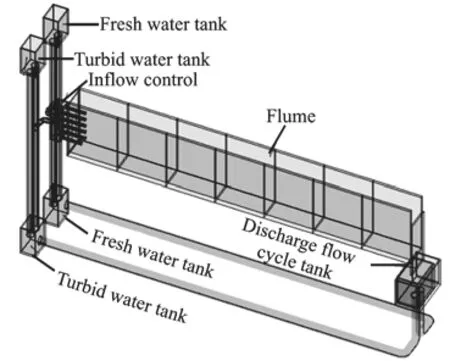
Fig. 1 Schematic diagram of laboratory flume

In all experiments, silica flour with a median particle diameter of 7 μm is used to produce the turbid water and the initial density of the turbid water is less than 1 002 kg/m3. Hence, the turbid water can be treated as a Newtonian fluid. A circulating water mixer is used in the turbid water underground tank,and after the silica sand particles are well mixed, the turbid water is released to the flume to form the density current. In experiments, the turbid water is pumped from the lower underground tank to the higher tank, passing through the pipe of 0.05 m in diameter and then is flushed into 0.20 m deep fresh water in the flume. The flow rate of the turbid water is measured through the Venturi meter, and experiments are conducted for the flow rate from 1 L/s to 2 L/s. A water gauge is set to measure the water level, as shown in Fig. 2. The entire water level varying process is recorded using a digital video.

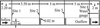
Fig. 2 Sketch of sample sites, the setup of sampling tubes and water gauges

As the water temperature influences the density of the fluid, two temperature loggers are used to measure the temperature of the fresh water and the turbid water. In the present study, the temperature of the turbid water is lower than that of the fresh water,with a temperature difference of approximately 10.2 C±°. A simple sampler is employed to obtain the water samples in different layers in the water column to analyze the vertical distribution of the sediment concentration. There are four sample sites and 31 sample points in the experiments, as sketched in Fig. 2.The site 1 has one sample point set at a place 0.10 m above the bottom, while the other sites have 10 sample points.

2. Mathematical model

2.1 Governing equations

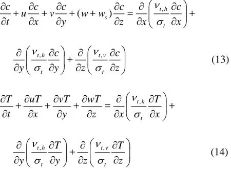
In the present study, the flows have relatively small density differences, the Boussinesq and hydrostatic assumptions are valid and are used in the simulations, and the following governing equations are to be solved:

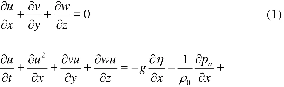
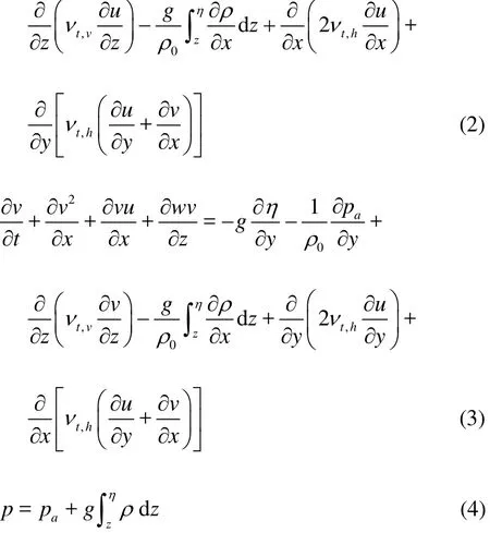
where u, v and w are the mean values of the velocity components in the directions x, y and z,p is the modified pressure,is the atmospheric pressure, ρ is the density of the mixture,is the reference density, η is the water surface elevation,g is the acceleration of gravity,is the horizontal turbulent viscosity andis the vertical turbulent viscosity.

In many numerical simulations, the small-scale turbulence cannot be resolved at the selected spatial resolution. In view of the density stratification, the buoyance influences the turbulent transport of both the momentum and the scalar quantities, and the unstable density stratification enhances the turbulent viscosity and the diffusivity. The turbulent viscosity contains two parts: the horizontal turbulent viscosityand the vertical turbulent viscosity. The horizontal turbulent viscositys modeled by using the subgrid models, such as the Smagorinsky model, and the vertical turbulent viscosityis modeled by using the -kε model.

By assuming that the subgrid turbulent energy production and dissipation are in equilibrium, Smagorinsky obtained the following expression for the turbulent viscosity, by expressing the sub-grid scale transport by an effective turbulent viscosity associated with characteristic length scale

wheresc is the Smagorinsky constant, l is the characteristic length defined as

where V is the volume of the computational cell.is the deformation rate defined by

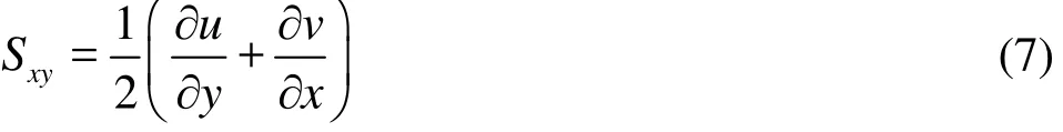
We have cs=0.2[20]. The vertical turbulent viscosity is determined by the parameters k and ε as

where cμis the empirical constant, k is the turbulent kinetic energy and ε is the turbulent kinetic energy dissipation rate. These two parameters are obtained from the flowing transport equations as:

wheretσ is the turbulent Prandtl number. The ranges of the empirical constants are listed in Table 1.

Table 1 Ranges of the empirical constants

In the present study, these parameters take the following values:with a good match with the experimental data[22], and=0.3 well in accordance with the density current.

The transport of the sediment and the temperature can be calculated using the following equation:

where c is the sediment concentration, T is the temperature andsw is the settling velocity of the sediment computed according to the Stoke’s law[36]defined as

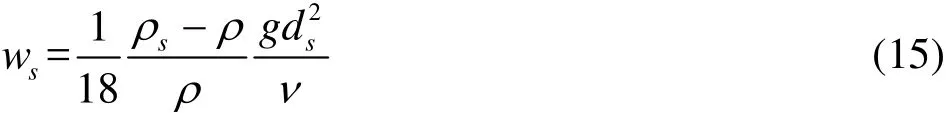
wheresd is the diameter of the sediment particle, ν is the viscosity of the fluid andsρ is the density of the sediment. In this model, the deposition termnear the bed is defined as

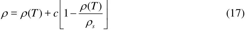
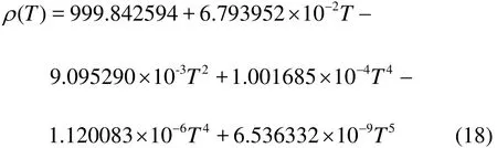
The influence of the sediment on the water density is expressed as

Table 2 Summary of experiment conditions of continuous (C) and discontinuous (D) density currents

2.2 Boundary conditions

In the experiments, the turbid water enters the flume at a certain velocity and concentration from the pipe at a zero angle with the horizontal plane, the velocity is set according to the inflow rateand the inflow duration tduration, and the concentration is set to the sediment concentration. At the inletthe von Karman constant κ is equal to 0.4, h is the water depth at the inlet and h = 0.2 m. At the free surface, the net fl uxes of the hor izontal mom entum and the turb ulent kin etic ener gy aresettozero.Thezerovelocitygradientnormalto the free surface is set, and the pressure is set to the atmospheric value. At the outlet boundary, a sharpcrested weir is employed, and the streamwise gradients of variables are set to zero. Hence, the outflow boundary is set at a certain distance downstream from the weir. At the rigid wall, the velocities are set to zero (u = v = w = 0), reflecting the no slip conditions.For the scalar equations, the gradients of the variables are also set to zero (? u / ? y = ? v / ? y = ? k / ? y = ? c/?y = 0) at the vertical walls. The initial temperature in the flow field and the temperature of the inflow are set to the ambient water temperature Tambientand the inflow temperature Tinlet(see Table 2), respectively.And the walls are set to be adiabatic with no heat transfer between the walls and the fluid.(the position where the inflow is cut off),

3. Results

The numerical results for the density currents from the continuous and discontinuous sources are compared with the experimental results in the laboratory. In Fig. 1, a 3-D view of the experimental flume is shown, and the parameters used in the numerical simulation based on the experimental data are listed in Table 2, including and the current arrival timearrivalt . In all experiments, the median particle size is 0.007 mm, and these particles have a density of 2 650 kg/m3. The total sediment concentration in the turbid water ranges from 0.3 kg/m3to 1.6 kg/m3.

3.1 Model performance for density current

In the present study, the mixing process is observed, and the sediment concentration against time is obtained. Figure 3 shows the time evolution of the sediment concentration at the observation point of the site 1, indicating that these model results are consistent with the experimental data, and this model can be used to predict the mixing process under the inflow conditions in the present study.

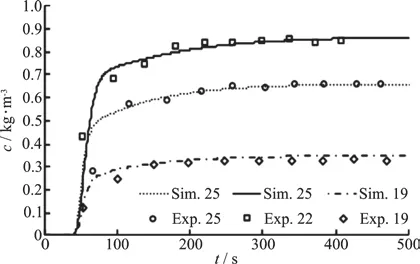
Fig. 3 Time evolution of sediment concentration at the sampling point of site 1

Figure 4 presents the surface elevation ()Hagainst time for the continuous and discontinuous inflows of 2.0 L/s. The data from the measurements according to a recorded video are consistent with those from the simulation, with differences less than 3%.

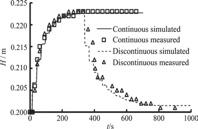
Fig. 4 Surface elevation in continuous and discontinuous cases against time

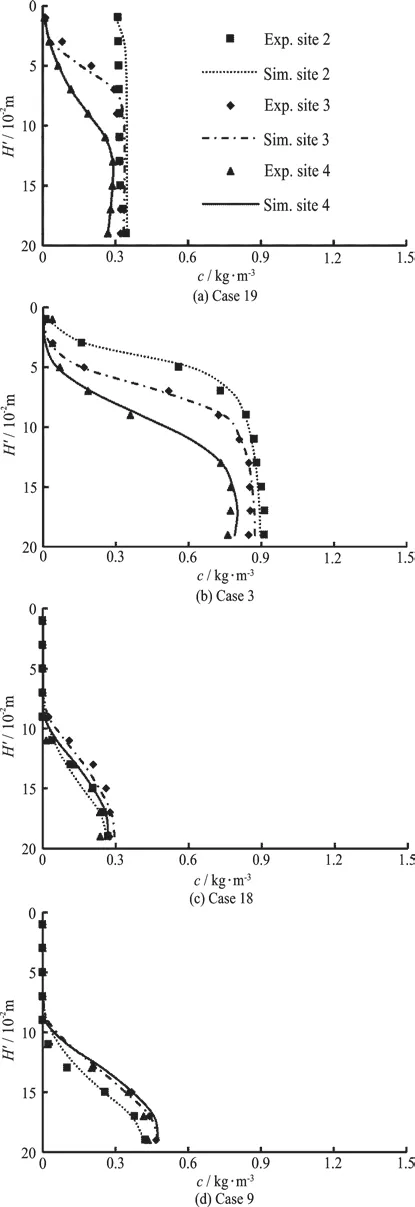
Fig. 5 Comparison of vertical sediment concentration c distributions between numerical results and experimental data of continuous currents

Table 3 compares the numerical arrival time with the experimental results and shows that the maximum absolute time error of the simulations relative to the experiments is 3.53%, and the minimum absolute time error is 0.94%, meaning that the experimental data and the numerical results are in good agreement. In these cases, the results as shown below can be obtained: (1) At early times, the currents of different sediment concentrations with the same inflow rate have almost the same speeds near the inlet, 0-5 m at 2.0 L/s and 0-8 m at 1.5 L/s, respectively. (2) At later times, the currents with a high sediment concentration move faster. (3) The turbid current front moves at almost a constant speed in the flume, except in the field near the inlet. It is evident that the above numerical model can be used to predict the front location of the density current and the change of the surface elevation.

The numerical simulation results are compared with the experimental measurements of the sediment concentration. Because the experimental hydrodynamics data are not available, the model hydrodynamics results could not be directly validated. Considering that the hydrodynamics governs the transport of the scalars, using inaccurate hydrodynamics data will provide an inaccurate sediment concentration. Therefore, good comparisons of the sediment concentration data between the experiments and the numerical simulations can indirectly validate the predictive capability of the model.

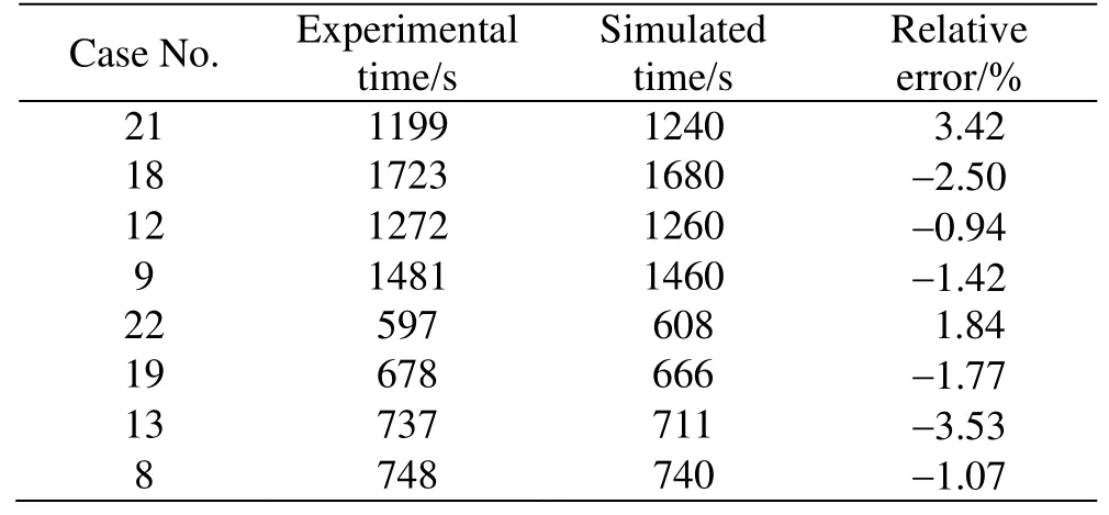
Table 3 Arrival time comparison between experiments and numerical simulations

Figure 5 shows the vertical sediment concentration distribution of the numerical results and the experimental data in different sites and different cases,where H′ is fixed water depth of sample point.Some obvious disagreements are observed, especially in discontinuous cases. Because the discontinuous density current differs from the continuous one after losing the energy supply from the inflow, and due to the complexity of the mechanism, the discontinuous density current is difficult to predict. Overally, the consistency of the simulations results with the experimental data is observed at most points, the numerical model results are reasonably consistent with the experimental data in continuous and discontinuous cases.

To further evaluate the rationality of the simulation results, the absolute mean error (AME) and the root mean square error (RMSE) are employed, as w

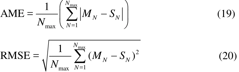
Figure 6 shows that the AME for the vertical sediment concentration is 0.026 kg/m3and the RMSE is 0.046 kg/m3over a range from 0 kg/m3to 1.2 kg/m3,and most scatters are plotted round the line =X Y with a correlation coefficient of 0.981, suggesting that the simulation results are consistent with the experimental data, whereMc is measured value,Sc is simulated value. In conclusion, the model mentioned above can provide a good prediction of the movements and the vertical sediment concentration profiles of density current.

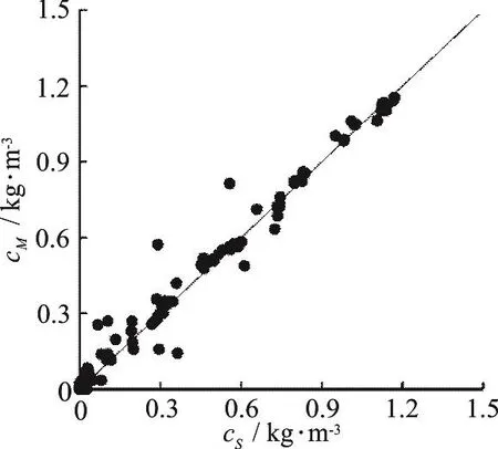
Fig. 6 Model performance for density current simulation

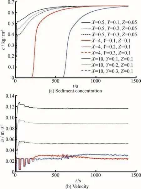
Fig. 7 (Color online) Time evolution of characteristic variables in case 25

3.2 Trend of characteristic variables in horizontal plane

To reflect the boundary conditions of the inflow from the pipe, a relatively strong turbulence flow field is generated near the inlet, and subsequently the sediment particles carried by the inflow are mixed with the ambient clear water, generating an ununiform field. Figure 7 shows the time evolution of the sediment concentration, the velocity u along the flume in the case 25, which obviously suggests that:(1) the sediment concentration will reach the same value, while the velocity remains stable and different across the section in the field near the inlet, (2) in the downstream field of the plunging point, the variables mentioned above are identical across section, (3) those variables vary greatly in the horizontal direction along the flume.

3.3 Characteristic differences between continuous and discontinuous turbidity currents

The vertical sediment concentration of the continuous turbidity current decreases from the plunging point to the front, and the thickness of the turbidity current shows the same trend, as it also decreases from the plunging point to the front (as shown in Figs.5(a), 5(b)). However, the vertical sediment concentration of the discontinuous turbidity current sees a completely different trend. The vertical sediment concentration and the thickness of the current increase prior to the site 3 and subsequently decrease (as shown in Figs. 5(c), 5(d)). It is obvious that the continuity of the inflow influences the vertical sediment structures along the bed. For the continuous turbid water inflow, the front has the energy supply from the tail to produce a turbulence to maintain the sediment particles in suspension and to overcome the friction from the bed and the interface to move forward. Without the continuous turbid water inflow,the current loses the energy supply and moves along the bed with the potential energy and the kinetic energy, while overcoming the friction. The movement of the current slows down, and the sediment carrying capacity of the current declines, and subsequently the sediment particles settle and deposit onto the bed.

Figure 8 presents the front velocityof the continuous and discontinuous turbidity currents, including also the time evolution of the front location. For the continuous turbidity current, the front velocity is almost consistent along the bed, with an average velocity of 0.03 m/s and an average acceleration of 2.9×10-6m/s2in the case 22. For the discontinuous turbidity current, the front velocity shows the same trend, as the continuous turbidity current in the early time. However, the front movement suddenly slows down and even stops after the inflow is cut off. In the case 21, the front shows an acceleration of 7.8×10-6m/s2.

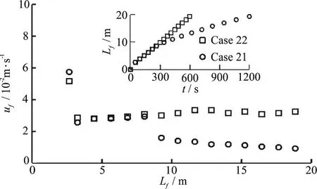
Fig. 8 Front velocity and time evolution of front location

Figure 9 presents the time evolution of the sediment concentration contour of the continuous and discontinuous turbidity currents. In the case 22, the interface of the turbidity water and the clear water shows an obviously positive gradient slope from the plunging point to the front. Hence, the height of the turbidity current falls along the flow path. As the turbidity current loses its energy supply from the inflow, the plunging point begins to fall back and subsequently vanishes. During this process, the potential energy of the dense water in the tail part transfers to the kinetic energy of the turbidity current for the current to go on moving forward with the particles in suspension. Therefore, the slope of the interface presents a negative gradient in the tail part and a positive gradient in the front part in the case 21.

4. Conclusions

Although the characteristics of the continuous turbidity current on a slope were extensively studied,no reports are available on the combined continuous and discontinuous turbidity current on a flat slope. In most previous studies, isotropic turbulence models were used, which can not accurately describe the anisotropic turbulence. In this paper, a model based on the Reynolds averaged Navier-Stokes equations and the scalar transport equation is developed to study the differences between continuous and discontinuous turbidity currents induced by low-density differences,unsteady inflow on a flat slope. The turbulence model combines the Smagorinsky model and the k-ε model and can capture the anisotropic turbulence.This model also takes account of the influence of the temperature and the sediment concentration on the water density, and the settling and deposition of the sediment particles. It is shown that the time evolution of the front location and the sediment concentration predicted using the model are consistent with the experimental data, and the results of the statistical analysis show that the AME value for the turbidity current is 0.026 kg/m3. Therefore, this model can be used to well predict the turbidity current. In addition,the following conclusions concerning the turbidity density can be drawn:

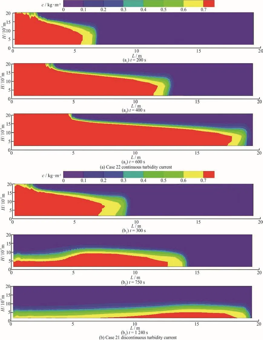
Fig. 9 (Color online) Time evolution of the turbidity current and sediment concentration contour

(1) At early times, the currents of different

sediment concentrations with the same inflow rate travel at almost the same speed, the currents move at almost constant speeds along the flume and the currents with high sediment concentration move faster at later times. In addition, the currents of higher,continuous inflow rate and sediment concentration move faster than those of the lower, discontinuous ones.

(2) The sediment concentration in the mixing zone becomes consistent. But the velocity and the turbulent kinetic changes greatly across the section and maintain the same in this area. The variables mentioned above are identical across the section in the downstream of the plunging point. Along the flume,the variables vary greatly.

(3) The vertical sediment concentration and the thickness of the turbidity current of the continuous turbidity current generally decrease along the flow path. However, the vertical sediment concentration of the discontinuous turbidity current sees a completely different trend, initially increasing and subsequently decreasing. These differences are induced by the complex energy conversion inside the turbidity current.

(4) For a continuous turbidity current, the front moves at an almost constant speed and a relatively low acceleration. However, for a discontinuous turbidity current, without the energy supply, the front movement will suddenly slow down after the inflow is cut off.