Exact Calculation of Antiferromagnetic Ising Model on an Inhomogeneous Surface Recursive Lattice to Investigate Thermodynamics and Glass Transition on Surface/Thin Film?

Ran Huang(黃然) and Purushottam D.GujratiState Key Laboratory of Microbial Metabolism and School of Life Sciences and Biotechnology,Shanghai Jiao Tong University,Shanghai 200240,China

2Department of Physics,University of Akron,Akron,OH 44325,United States

1 Introduction

Glass transition on surface/thin fi lm has drawn intensive interests in the last decades for two reasons:Firstly,the importance of surface and thin fi lm in materials science and engineering requires a better understanding of its dynamic and thermodynamic properties;Secondly,the con fi ned geometry is a good approach to understand the mysterious glass transition itself,especially to explore the dynamic properties within the thin fi lm geometry.Numerous works of both experimental and simulation/calculation approaches have been done on glass transition on surface/thin fi lm.[1]

Keddie and co-workers firstly investigated the supported thin fi lm of polystyrene(PS)by ellipsometric measurements.[2]They prepared several PS fi lms supported by silicon wafers with thickness from 100?A to 3000?A.The measurements indicated the deduction of the Tgwith thickness under 400?A.An empirical relationship between thickness and Tgwas given as:

whereis the glass transition temperature of the bulk PS.The parameters α and δ are fi tted to be 32and 1.8 respectively,h is the thickness of the fi lm.Following Keddie’s work,many researches have been conducted on supported thin fi lms of various polymers[3?4]by different characterization methods,e.g.X-ray re fl ectivity,positron annihilation,and dielectric measurement.[5?7]Most results have demonstrated the same phenomenon that for liner polymer the Tgdecreases with the thickness of fi lms.However the supported fi lm has a considerable fi lm-substrate interaction,which makes the conclusion controversial.Strong attractive interaction between the substrate and thin fi lm may increase the Tgof thin fi lm above the bulk Tg.[7?8]Forrest and co-workers have done pioneer works in measuring the Tgof free-standing thin fi lms.[9?11]Their results showed that the Tgdecreases with the thickness of PS thin fi lm with a much larger magnitude:for example,the Tgof 200?A fi lm with molecular weight(Mw)within 120 K to 378 K reduces by 70 K below thewhile this magnitude is around 10 K for supported fi lms.The empirical equation(Eq.(1)) fi tted for supported fi lm still holds for the low Mw free-standing fi lms.With δ=1.8,the parameter α was found to be 78,which is roughly twice of it found for supported fi lms.

Other than the experimental works,computer simulation and calculation have also been developed to investigate the glass transition on surface/thin fi lm.[12?24]Molecular Dynamics(MD)and Monte Carlo(MC)method were usually employed with various modelings,and con fi rmed the Tgdecrease with the thickness reduction for both supported and free standing fi lm,or Tgincrease in some particular substrate- fi lm cases.Equation(1)derived from experiments can also be validated by simulations,nevertheless the explanation for the mechanism of Tgreduction is still a matter of debate.Most MD simulations veri fi ed the experimental observation that for supported fi lm,a strong substrate- fi lm interaction will increase the Tgabove the value in the bulk,while the weak substrate- fi lm interaction will lead Tgreduction,and freestanding fi lm shows a much larger Tgreduction than supported fi lm with weak substrate- fi lm interaction.[13]Mattice and co-workers firstly reported the MC simulation in this field.[14?15]Basically the Tgreduction with smaller thickness was con fi rmed and fi tted by Eq.(1)in the above investigations.

Although the glass transition is not a unique property of polymers,since it is more concerned in the polymer community and almost all experimental works were on the polymeric systems,most simulations and computations were also modeled for polymers,while the works on small molecule systems are very rare.Meanwhile,Ising spin glass has also been widely utilized to study the glass transition.[25?38]By different lattices adopted and interactions setup,the Ising model is capable to describe various systems,such as gas,liquid,crystal and glass,and consequently the phase transitions,like melting and glass transition.[25]However,very few of the e ff orts were conducted on surface/thin fi lm glass transition of Ising spin glass.This field had been explored by Gujrati etal.by applying Ising model on a modi fi ed Bethe lattice to describe the thermodynamics of polymer systems near surface.[39?43]In this paper we follow the similar methodology to study the glass transition of Ising spins on the surface/thin fi lm on a specially constructed recursive lattice.

2 Surface Recursive Lattice(SRL)Geometry

Except in some rare cases,[44?46]a many-body system with interactions on a regular lattice is difficult to be solved exactly because of the complexity involved in treating the combinatorics generated by the interaction terms in the Hamiltonian when summing over all states,and the mean- field approximation is usually adopted to solve this problem.On the other hand,recursive lattices,e.g.the Bethe lattice,enable us to take the explicit treatment of combinatorics on these lattices and then no approximation is necessary.[28?36]The recursive lattice is chosen to have the identical coordination number as the regular lattice it is designed to describe.As usual,the coordination number q is the number of nearest-neighbor sites of a site.A typical recursive lattice,the Husimi lattice,as the analog of 2D square lattice is shown in Fig.1.

Since the methodology of recursive lattice is to approximate the regular lattice,almost all the previous studies in this field were merely on in fi nite and homogeneous recursive structures,and such modeling can only be applied to the bulky systems.In this work we construct a recursive lattice to describe the surface/thin fi lm.This so-called surface recursive lattice(SRL)is inhomogeneous with various unit cells,and has a locally fi nite-sized geometry to mimic the 2D case,i.e.the 2D bulk with 1D surfaces.The SRL is integrated of square units representing the bulk and single bonds representing the surface,the structure is made to have the same coordination numbers with regular 2D square lattice.Ising spins will be applied on the lattice sites to represent a small molecule system.The exact calculation will be derived and the solutions will be discussed.

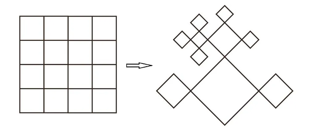
Fig.1 A regular square lattice and its analog of a recursive lattice(the Husimi lattice).

2.1 Construction of SRL

(i)Structure

To approximate the regular lattice due to the identical coordination number,we firstly need to fi gure out the coordination number and interactions of a regular lattice of surface/thin fi lm to construct the SRL.Figure 2 shows a regular 2D square lattice of a thin fi lm with thickness of 5,with the thick bonds representing the surface.(We will take thick bond to represent the surface bond through this paper.)Here we label the central layer to be the 0-th level,and the layer next to 0-th layer is the 1-st level.The surface layer is labeled as level S.The sites on the surface have coordination number of 3,while inside the bulk the coordination number is 4.Analogically,a hybrid recursive lattice with q=3 and 4 is required to describe the surface/thin fi lm.

Now we take out the basic units inside the bulk and on the surface to construct a recursive lattice.Inside the bulk we simply have Husimi square lattice of q=4.For the surface structure,a single bond representing the surface links on a square unit then we can have sites with q=3.However this unit cannot be simply adopted to construct a recursive structure,because the recursive calculation technique(will be detailed later)requires an origin point,to which the entire tree is symmetrical.For the unit shown in Fig.3(a),wherever we determine the origin is(point A or B),the unit is not symmetrical to that point.We modify the surface unit by replacing one square with an arti ficial single bond at one lower corner,then the modi fi ed unit(Fig.3(b))is symmetrical to the point A.Although this unit di ff ers from the regular lattice we mean to approximate,the coordination numbers on the surface square still accord to our design and calculation in the following sections will show that this approximation is practical.

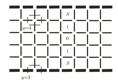
Fig.2 A regular 2D square lattice of a thin fi lm with thickness=5.

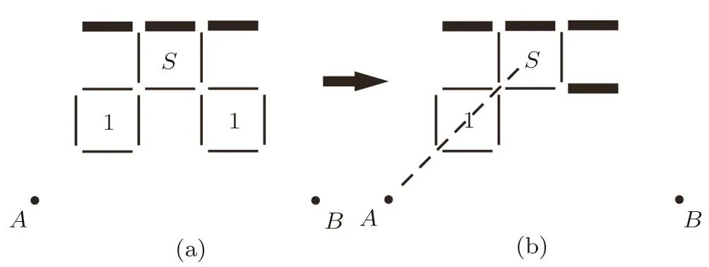
Fig.3 The modification of surface square unit.The bulk square on lower right corner is replaced by a single bond.In this way the modi fi ed structure is symmetrical to an imaginary axis linking point A and the center of square unit S.

Hence we can put the bulk and surface units together to construct a recursive lattice to approximate the regular thin fi lm lattice.The structure of a thickness=5 lattice is shown in Fig.4.From surface A to B,we have a finite bulk portion with thickness=5,and these fi ve layers are labeled as S,1,and 0 like the regular fi lm lattice in Fig.2.The thick single bond representing surface links two identical bulk trees.In this example,one bulk tree TBis linked overall with another 36 trees(only one of such linked-trees is drawn in Fig.4),while they are all identical and independent with each other except a single surface bond connection.Recursively,each of these 36 trees is also linked with another 35 trees by single surface bonds.This lattice is an in fi nite tree integrated by fi nite-sized bulk portions and in fi nitely large surfaces.If we look at the surface integrated by thick surface bonds indicated by the arrow at the right lower corner in Fig.4,we can see the surface going through the bulk trees TBis in fi nitely long with q=3 everywhere.A stretched surface is shown in Fig.5 to provide a more obvious view.Comparing to the regular lattice,the main di ff erence is that one surface also receives thermodynamic contributions from other surface structures,which is caused by the surface unit modi fication.But this is an approximation we have to adopt to achieve the recursive calculation.Although we have in finite number of bulk trees and surfaces in this lattice,since they are independent and identical,it does not impact the thermodynamic properties of a local region we are going to investigate.

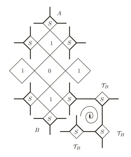
Fig.4 A bulk tree structure in surface recursive lattice with thickness=5.

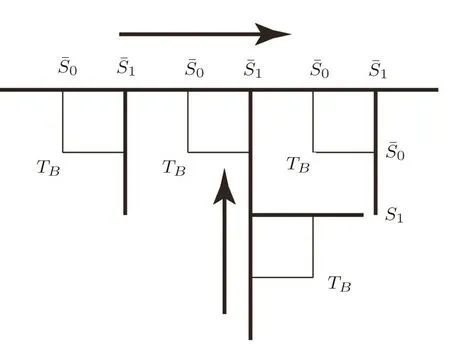
Fig.5 The stretched view and the contribution direction of one surface in SRL.The surface sites are labeled in a recursive manner.

(ii)The Sites Labeling on Bulk and Surface Units

We label each site in a square as shown in Fig.6.The label is in a form of Sa,b,where a is the index of the square unit in the bulk tree,and b is the index of site.Therefore,one site Sa,bactually has two labels depending on which square unit we refer to.For example the site Sa,4is also S(a+1),1in the unit on higher level.When we are only focusing on one unit,the site Sa,bcan be denoted as Sbfor convenience.In a square unit,the base site is determined to be the site closest to the bulk tree origin(The 0th square)and labeled as Sa,1.Therefore,in the upper enlarged circle in Fig.6,the base site is the lowest site,while in the lower enlarged circle,the base site is the left one.The labeling in the origin unit is a special case which will be discussed later.The interactions are also sampled in the enlarged circle:J is interaction between the nearest sites,Jpis interaction between the second-nearest sites,i.e.the diagonal sites.

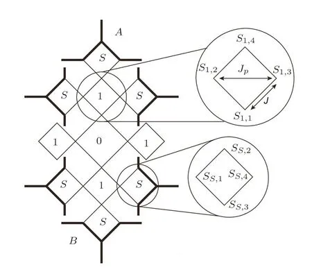
Fig.6 Sites index on a square unit in SRL.

For surface calculation,we label the surface sites as shown in Fig.5.Due to our calculation method,only two labels are necessary in surface labeling.The site close to the bulk site is labeled asˉS0,and the site diagonal to the bulk site is labeled asˉS1.

(iii)The Interactions and Energy in Bulk Square Unit

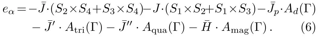
Besides J and Jp,we also consider the other two types of interactions in our model:J′the interaction energy of three sites(triplet),and J′′the interaction energy of four sites(quadruplet).We introduce the following variables to count the interactions and magnetic fields of one square unit:

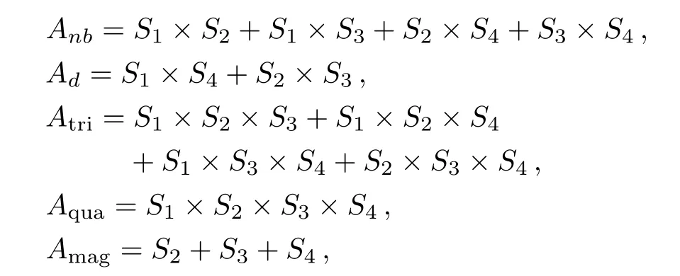
where Smis an Ising spin with the value of±1.Note that the base site S1is not included in the magnetic term Amag,because the calculation has a recursive fashion that the energy of one unit is contributing to the unit on next level,and the base site of one unit will be counted as the top site in the next level.

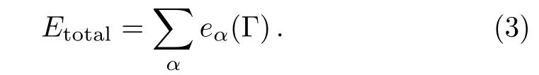
For a particular cell α with a certain spin conformation Γ,the energy of one cell in the model is:

and the total energy of the Ising model on SRL is sum of the energies of all cells:

In this work Jis negative to adopt the antiferromagnetic Ising model,the neighbor spins preferring different states corresponds to the lowest energy stable state,i.e.the ordered crystal conformation,which has the largest weight comparing to other conformations at the same temperature,while the neighbor spins of the same states is the most unstable conformation with the highest energy,which represents the disordered phase.

The Boltzmann weight ω(Γ)of state Γ is given by

where β=1/kBT is the inverse temperature,and we set the Boltzmann constant kB=1 to generalize the temperature to be in the unit of energy.

Then the partition function of a fi nite lattice with α cells is the sum over products over the Boltzmann weight:

(iv)The Interactions and Energy on Surface

In Fig.5,the single bond unit and the square unit alternatively appear on the surface structure.The interactions and energy of the surface square unit are similar to the bulk square unit as we discussed in previous section.However,here we would like to assign a different nearest neighbor interactionon the surface bond,to distinguish it with J in the bulk.This enables us to investigate more complex surface properties.And similarly we may also have a different diagonal interaction(),triplet(),quadruplet(),and magnetic field():

On the surface single bond unit,the interaction is much simpler since there is only one nearest neighbor interaction:

Similar to the role of base site in bulk calculation,here the magnetic field ofˉS0is not included in the second term because that site will be counted in the next level’s energy equation.The “l(fā)evel”,in this statement,is indexed by taking the direction indicated by the arrow in Fig.5,and employing an imaginary origin point in fi nitely far away from the region we concern.Since the surface is in fi nitely large,the selection of“origin point”does not a ff ect us to achieve the solutions on surface.

By the setup of interaction energy parameters,we can simulate various systems with particular interactions and energy to study their thermodynamics and phase transition with the determination of the partition function.We will generally set J=?1 to determine the temperature scale for our model.The solution based on J=?1(=?1)and all other parameters to be 0 is called the reference model.

2.2 General Recursive Calculation Technique

Although the recursive calculation techniques have been well discussed in previous works,[28?38]here we brie fl y review the general approach on recursive lattice for a better understanding the methodology developed in this work.Firstly we introduce the concept of sub-tree contributions.In the fi nite bulk tree we have an origin site at the center of the bulk.For each square unit,the base site is the closest site to the origin,and there are three subtrees coming from the other sites.The sub-trees could either be three identical portions of the bulk tree,or three surface trees linked by the single bond if it is the square unit on the surface.We label the levels in one unit and show the sub-tree contributions in Fig.7.

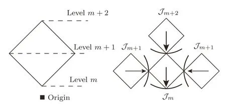
Fig.7 The levels on a square unit and the sub-tree contribution.

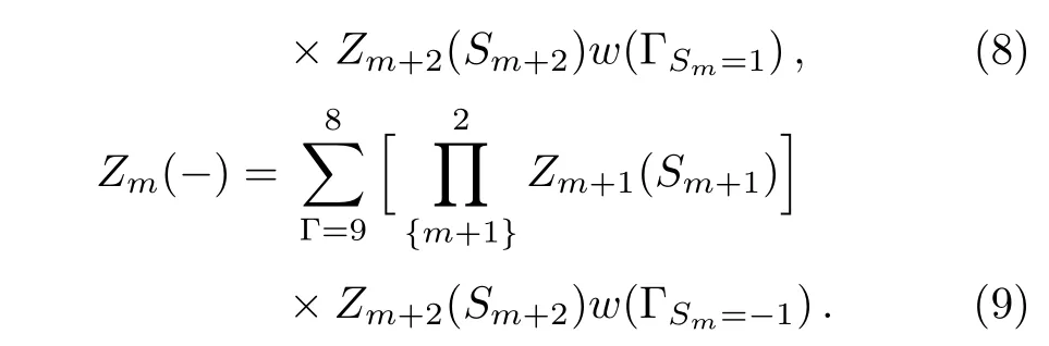
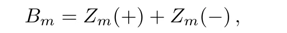
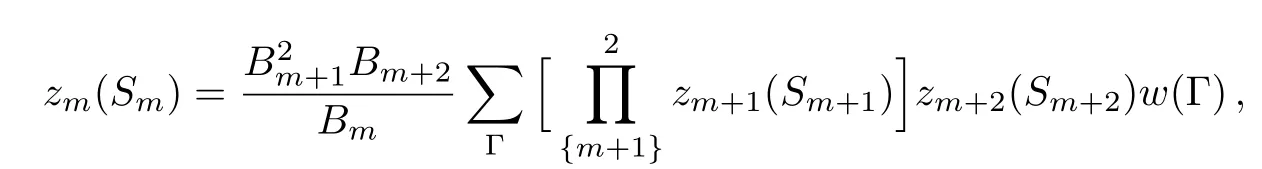
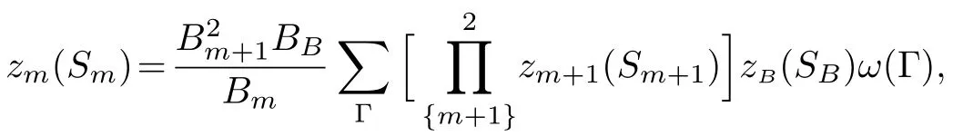
By this index,the sites on the level m are represented as Sm.The sub-tree going to the site on level m is marked as Tm.In this way,we can introduce the partial partition function(PPF)Zm+1(Sm+1)at the level m+1 to represent the contribution of the branch Tm+1with a certain state of spin Sm+1as its base site to the lower level m,and Tmto the lower level m?1,etc.Therefore the PPF Zm(Sm)at level m is a function of the PPFs Zm+1(Sm+1)and Zm+2(Sm+2)at higher level m+1 and m+2 and the local weight.Then we can start from the highest level,count the contributions of sub-trees on each level and recursively go to the lower level unit,and finally to the origin point,where it gains the contribution of the entire lattice,and the thermodynamics of the whole system can be obtained by the partition function.The PPF Zm(±)of a sub-tree Tmis the sum of the con figurations with the spin Sm=±1 over the products of the PPFs on higher levels with the local weight ω(Γ).For a square unit,Zm(+)has 8 terms with Sm=+1 and Zm(?)is the sum of the other 8 con figurations with Sm=?1:

Depending on the spin state(S0=±1)of the origin site,the two sub-trees’contributions to the whole system are:

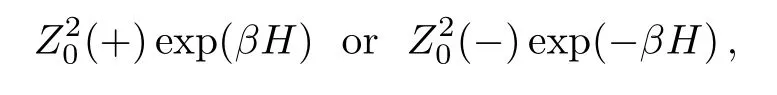
where the magnetic term is to count the contribution of origin site which is not contained in Eq.(2).The partition function Z0of the entire lattice can be accounted by the contributions to the origin site:

The first term is to count the conformation with the origin site spin S0=+1,the square of PPF represents two sub-trees and the weight of the origin spin itself is counted as exp(βH),similiarly for the S0= ?1 situation in the second term.

Or,if the origin is de fi ned to be a square unit,the partition function is

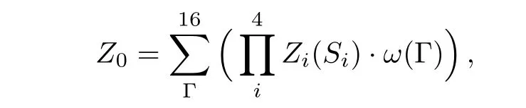
where Siis one of the four spins on the origin square,Zi(Si)is the PPF of the sub-tree coming into the site Si,and w(Γ)is the local weight of the origin square.

Then we can introduce the ratios

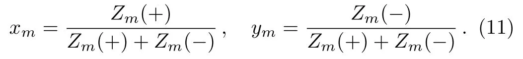
These two are the ratios of PPFs on the level m;they indicate,although not exactly to be,the probability that the site Smon level m is occupied by a plus spin(xm)or a minus spin(ym).Therefore,these two ratios,which we call the solutions,are critical in our model and all the thermodynamic calculations are based on the solutions.

De fi ne a compact notation for convenience:

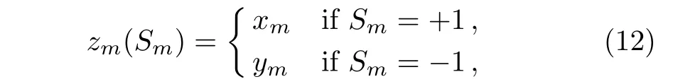
by introducing

we have

Substituting these two equations into Eqs.(8)and(9)leads to

where the sum is over Γ =1,2,3,...,8 for Sm=+1,and over Γ =9,10,11,...,16 for Sm= ?1.It is clear that the solution(ratios)on one level is a function of the solutions on higher levels in a recursive fashion.

For convenience,we introduce the polynomials:

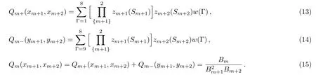
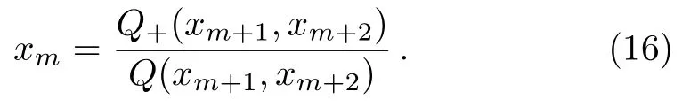
Then the ratio xmis simply a function of the ratios on higher levels xm+1and xm+2:

From the recursive relation shown in Eq.(16),we may expect a repeating solution,which has the form:x1,x2,...,xv(xv≥1)and xk=xv+kfor some value of v≥1,so that Eq.(16)holds.

Such a solution can be called a v-cycle solution that repeats after the v-th application of the recursive relation equation.For instance,with a 1-cycle solution x,we simply have the same ratio x on all the levels

For a 2-cycle solution x1and x2we have

That is,the two solutions alternatively appear by succeeding levels.In this way,for a particular recursive relation,we can start from a set of initial seeds x1and x2to calculate the solutions on lower levels until we reach the recursively repeating solutions,which is called fi x-point solution.Usually many initial seeds are tried to obtain all the possible solutions for a particular recursive relation.According to our experience,in the lattices discussed in this work,solutions with v≥3 were never obtained,while solutions with v=1 and v=2(1-cycle and 2-cycle solutions)are almost always available.Based on the property of x,which determines the probability that one site is occupied by the plus spin,a cycle solutions with v≥3 is hard to imagine.For the details of 1&2-cycle solutions of the bulk Husimi lattice,please refer to our previous works.[35,37]

2.3 Recursive Calculations on the Surface Lattice

(i)Calculation in the Bulk

For an in fi nite Husimi lattice,the calculation to get the fi x-point solution is straightforward,[35?38]we can simply start with two arti ficial initial seeds and recursively calculate the solutions by Eq.(16) fi nite times till reaching the fi x-point solution.While the case is quite different for the SRL we developed in this paper,the bulk tree is fi nite and con fi ned within surface trees,we need to carefully monitor the calculation on each speci fic site.

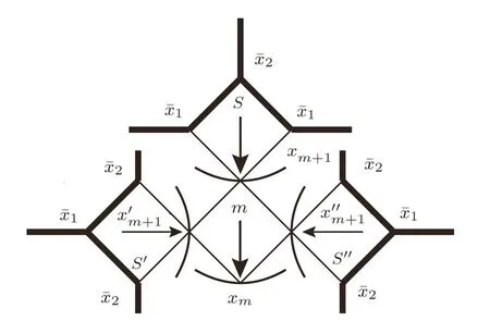
Fig.8 The initial seeds calculation scheme starting from the surface in SRL.

Let us take an SRL with thickness of 2m+3,we label the surface square as S,then the square next to S is labeled as the m-th level,then origin square is labeled as 0.Firstly we start from two initial seedsandon the surface sites as shown in Fig.8.The calculation on the surface square S provides the solution xm+1on the top site of m-th square.On the other two surface squares labeled as S′and S′′we use the same initial guess seeds,however rotate their positions by puttingon the top site andon two side sites,then the calculation based on S′or S′′will provide the solutionon the side sites of level m-th square.This is because for the anti-ferromagnetic Ising model and the properties of 2-cycle solution introduced above,we expect a 2-cycle style solution on our lattice(and the 1-cycle solution is just a special case when the two 2-cycle solutions are the same),thus the rotation avoids us to get the same results on neighbor sites,which makes the 2-cycle solution impossible.

Consequently,with the solutions xm+2and xm+1we obtain xmon the top site of square level m?1,and on the other branch the rotation of xm+2and xm+1will give us xm?1,then we can continue the calculation to the origin square 0 as shown in Fig.9(a).

Once we reach the solution x1andat the origin square,we have the states inside the bulk if the solution is the fi x-point one.This part of calculation is called downward calculation,which is from the surface to the bulk origin.However,this set of bulk solutions is from the initial guesses on the surface;it may not be the solution of the real state.We still have to find the fi x-point solution on the surface,and the bulk calculation from the surface fi x-point solution is then the final result we are looking for.To find the fi x-point on the surface,we start from the bulk origin and trace back to the surface(upward calculation),which provides a bulk contribution TBto the recursive calculation on the surface.

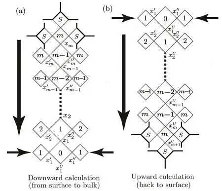
Fig.9 The calculation direction though the bulk tree:(a)start from surface to the bulk origin,(b)start from the bulk origin and go back to surface.

The upward calculation is shown in Fig.9(b).At the origin square,from the contributions of three identical trees and the local weight of the origin square,we can calculate the solution on the lower site,which is labeled as(Index U stands for“upward”).Then fromand so on.The upward calculation will provide the solutionat the base site of the surface square unit.This solution will be used as xBrepresenting the bulk e ff ect to surface in the surface calculation.

(ii)Calculation Along the Surface

The situation on surface is more complicated than in the bulk.From the previous introduction on downward and upward calculation,we can see a hint that depending on the direction of calculation,the solutions might be different on the same site,for example the xmandare different even they are on symmetric sites to the origin.This direction issue does not a ff ect us to explore the solutions describing the bulk,however it is critical in surface calculation.Therefore,we firstly classify two directions on the surface with speci fic labeling,as shown in Fig.10.

In Fig.10,the labeling on the surface is in this way:the solution on the base site is xB,which is thefrom upward calculation;the solution on the sides of the square is label asˉx1,and on the top isˉx2;the prime marks the direction that goes out from the square,while the label without prime is the direction going into the square.The scheme A shows a “side-to-top” direction:the solution going out from the top site,,is calculated from the solution going into the side siteand the base site solution xB.Then fromwe go through a single bond to get the next.The scheme B shows a“side&top-to-side”direction:the solution going out from the side site,,is calculated from the solution going into the side site,the solution going into the top site,and the base site solution xB.Again fromwe then go through a single bond to get the next.Only after we have done the calculations in both directions,we can get the surface solutions pair,the solution going into the top site,and the solution going into the side site,to do the subsequent bulk calculation.(Note that initially this pair is a guess we made to do the first iteration’s bulk calculation).The surface calculation scheme is shown in Fig.11.

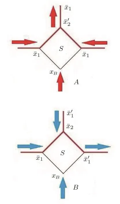
Fig.10 (Color online)Two calculation directions on the surface of SRL.

The upward bulk calculation provides us the bulk tree contribution and the solution xBon the base site of surface square.This solution can be taken as a constant in the surface recursive calculation.In Fig.11,we start from the xBand the initial seedto do two calculations as mentioned.The recursive calculation in process A will eventually give us a fixed,while the process B will give us a fixed.This new fixed set ofandis then the seeds we are going to use for the next iteration’s bulk calculation.Note one di ff erence in process A and B is that in process A we only needfor calculation,which is updated step by step,however in process B after each step we will only have an updated,whileis a constant in calculation.Thus,in practice we always do the process A first to get a fixed,then use thisas a constant in the calculation of process B.

The calculation on the square unit,for example,in process B,is the same as the bulk calculation.The calculation through the single surface bond,for example,in process B,is also similar with the square.The di ff erence is that the PPF only has two terms since there are 4 con figurations of a single bond structure:

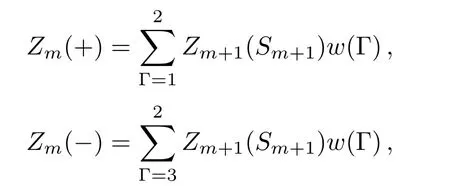
where the sum is over Γ=1 and 2 for Sm=+1,and over Γ=3 and 4 for Sm=?1.Then we have the polynomials:

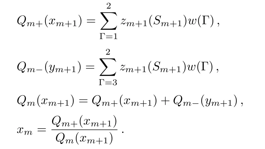
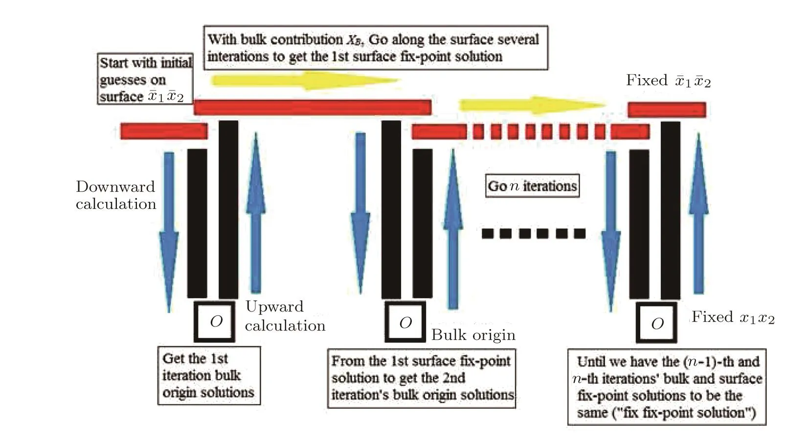
Fig.12 (Color online)The calculation process scheme to reach the fi x-point solutions in SRL.The vertical process is calculations through bulk tree and the horizontal process is along the surface.

The calculation scheme to reach the fi x-point solutions both on the surface and in the bulk is shown in Fig.12.We do an embedded recursive calculations to obtain the final solutions on the surface and in the bulk.The n iterations provide us recursively updated solutions in the bulk until we find the fi x-point solution,and a recursive calculation along the surface is embedded in one iteration to take the e ff ect of updated bulk contributions each time.This process is to make sure that we counter the mutual e ff ects from surface to bulk and from bulk to surface.Another necessity of this complicated process is that the bulk tree has a fi nite size thus the fi x-point solution is not guaranteed to be reached during one downward calculation.For the structure with thickness≥19,we can always obtain the fi x-point solution at bulk origin,although on the first several layers close to surface we can only have numerical calculations instead of exact solutions.(This“numerical depth”depends on the energy parameters setting and it shows always being smaller than 19 according to our experience.)

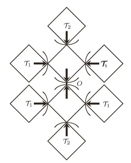
Fig.13 The sub-tree contributions to the origin point.

3 Calculation of Thermodynamics

3.1 General Free Energy Calculation Method:the Gujrati Trick

Since our lattices are in fi nitely large,it makes no sense to calculate the partition function or free energy for the entire lattice.However an exact treatment called Gujrati trick has been well developed to deal with the thermodynamic calculation on recursive lattices in our group’s previous work,[29,35,47?48]by this technique we can approach the thermal properties in a local area(per site)by the PPF Z(S)and solutions x we discussed in the previous section.

Here we take a regular Husimi lattice as an example to introduce the thermal calculation derived from partition functions.Recall Eq.(10),since Z0counts the contribution of the whole system,it must be the sum of contributions of the six sub-trees on level 1 and 2,and the weight of the two local square units on the origin.If we cut o ffthe two sub-branches on level 2 and joint them together,we will have an identical but smaller lattice.Similarly the partition function of this smaller lattice is:

We also cut o ffthe 4 sub-branches on level 1 and form two smaller lattices and their partition function will be

As an extensive quantity the free energy of the whole system is the sum of the free energies of these three smaller lattices and the two local squares:F(Z0)=2F(Z1)+F(Z2)+F(Zlocal).

This yields

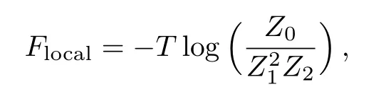
as the free energy of the two local sqaures,i.e.four sites(three paris of half-sites and the origin site).

The free energy per site is:

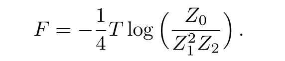
By substitutingZm(+)=Bmxmand Zm(?)=Bm(1?xm),we have

recall that for either 1-cycle or 2-cycle fi x-point solutions we have x0=x2,and Q0=

It follows

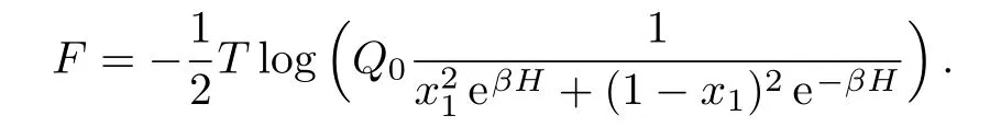
With the calculation of Q0and fi x-point solution x0and x1we discussed in the previous section,the free energy can be easily achieved.And the entropy is the first derivative of the free energy with respect to the temperature:

With the free energy and entropy we have the energy per site(energy density)as

A typical thermodynamic behavior of a Husimi square lattice with J=?1 and all other parameters to be 0 is shown in Fig.14.The free energy of two solutions are identical at high temperature.At the melting temperature Tmthe 1-cycle’s free energy di ff ers from 2-cycle’s and is less stable.The continuous entropy at Tmof 1-cycle implies the supercooled liquid state,while the entropy decrease of 2-cycle state implies the crystallization.Although here the entropy decrease is not a discontinuous jump as the typical behavior of first order melting transition,we may still treat it as the phases-coexisting point since the 2-cycle state is the most stable state here.

Thethermodynamicsof1and2-cyclesolutions agree with our anti-ferromagnetic model.The antiferromagnetic Ising model prefer to anti-aligned neighbor spins,therefore the 2-cycle state should have the lowest energy,i.e.the crystal,while the 1-cycle solution represents the metastable state with higher energy.With continuing the cooling process we can observe that at T=1.1 the entropy of 1-cycle state(supercooled liquid)quickly decreases to zero and becomes negative.This is the Kauzmann paradox and the ideal glass transition.The negative entropy is unphysical thus the metastable state must undergo a transition to be the glass state at TK,the ideal glass transition temperature.The free energy of the glass state below glass transition temperature is indicated by the last legend in Fig.14.Note that this branch is not provided by the calculation,instead it is a theoretical expectation.

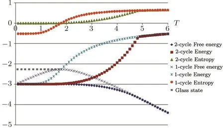
Fig.14 The thermodynamic behavior of a Husimi square lattice with J=?1 and all other parameters to be 0.

3.2 The Gujrati Trick Applied on the SRL

Although the basic principle is the same,asymmetrical structure of SRL requires further complex tricks to achieve the calculation.If we take a random site on the surface as the origin,to do the “cut and re-joint” trick we need to select a local region around this origin,and find matching sub-trees contributing to the local area.Here the matchings are more speci fic than they are in a homogeneous bulk lattice.For example in the Husimi lattice discussed in previous section,all the sites are identical,thus if two sites have the same solution x on them,the sub-trees cut o ff from them can be joined together to make a new lattice.However,the sites on the surface of SRL have three different situations:on the top of a surface square where the sub-tree’s contribution going out,on the side of a surface square where the sub-tree’s contribution coming into,and on the bottom of a surface square where the bulk tree’s contribution coming into.The matchings must be done on sites with exactly the same situations to make an identical but small lattice,but the asymmetrical structure of SRL makes the cutting and matching impossible.Wherever we select the origin local area and cut the sub-trees,there will always be two sub-trees left and cannot be matched with each another.

Figure 15 shows two failure cutting schemes,with“1 square and 2 single bonds” area and “2 squares and 4 single bonds”area respectively.In the cutting scheme#1,by removing the local area surrounded by the discontinuous curve,we have four sub-tree at the point A,A′,B and B′.The two sub-trees on A and A′can be linked together to form a smaller lattice with exactly the same structure.While the sub-trees on B and B′do not match with each other,since they are a bulk sub-tree on B and a surface sub-tree contributing the top site of a surface square.

In the cutting scheme#2,the local area of“2 squares and 4 single bonds”is bounded by the dot curve.The sub-trees on C–C′and D-D′can form smaller lattices.Although the new formation of D–D′is not identical to the entire lattice,we can still count its partition function and handle the ratio calculation.However the same difficulty,as we encountered in scheme#1,presents on the sitesEandE′:TheEsite is at the side of a surface square while theE′site is on the top.

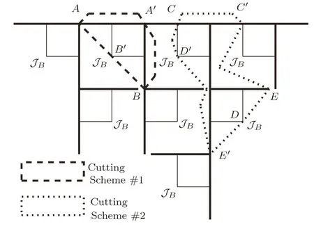
Fig.15 Two example failure cuttings in SRL.

Therefore,either we choose odd or even numbers of basic units as the local area around origin,the Gujrati trick cannot be done.We have to somehow modify the origin structure to avoid the problem of asymmetry.As shown in Fig.10,the single bond and square unit have a“head-to-side” connection,that is,following the calculation direction,the sub-tree coming from a single bond is always linked to the side site of next level’s square,or vice versa.This arrangement is designed to make the structure uniform on the surface,but it also causes the asymmetry.It is necessary to make one“head-to-head” connection as the origin of the surface,as shown in Fig.16.

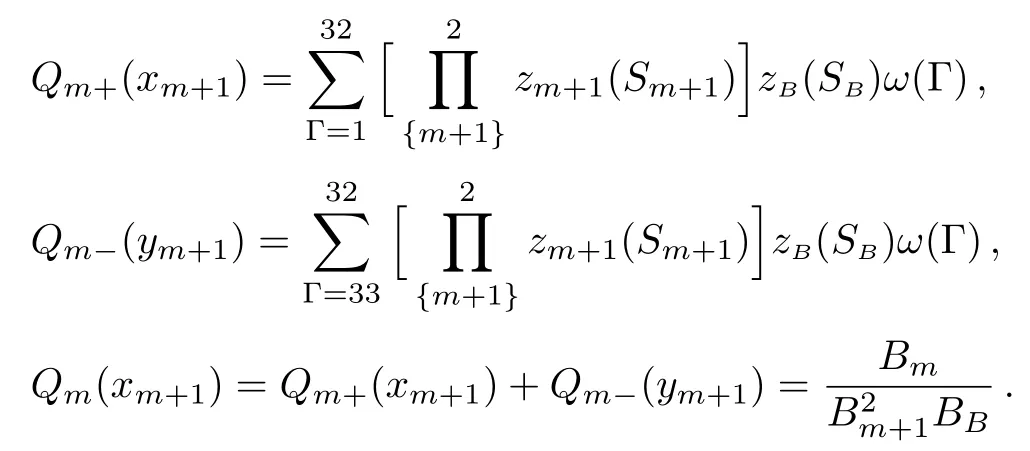
In this way,we have two in fi nite and identical surface trees connected in a“head-to-head”style,then this single bond is the origin of our entire lattice,and except this bond,all other surface single bonds are in “head-to-side”connection.Starting from the origin,the closest squares can be labeled as level 1;the second closest squares are on level 2 and so on.As shown in Fig.16,by the selection of four squares and six single bonds as the local area,we can form one identical lattice on level 1 at the sites A–A′,two identical lattices on level two at the pairs B–B′and C–C′.The sub-trees cut at D,D′,EandE′are identical bulk trees so we can pair them to form two bulk lattices.Now we can easily derive the free energy of the local area to be:

Unlike the point origin in Husimi lattice,here the origin is a single bond unit.The total partition function thus has four terms due to the four possible states of the single bond:

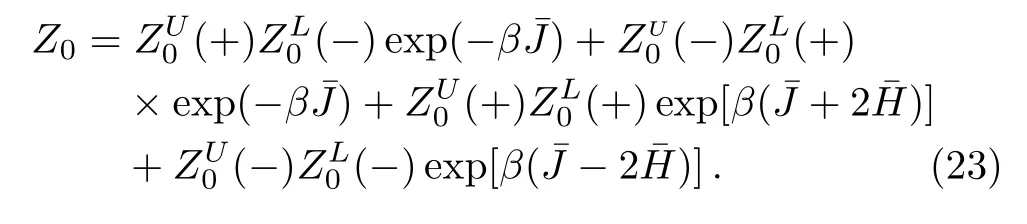
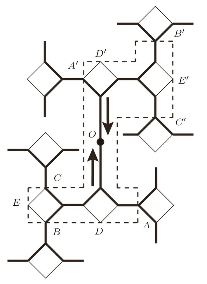
Fig.16 The modi fication on the surface of lattice and the cutting area around the origin.

To speci fically track the spins in the origin area and rematch the sub-trees,we de fi ne the two sub-trees meeting at the origin bond as “upper” and “l(fā)ower” parts.In Eq.(23),the superscript U or L is to indicate the upper or lower part of the lattice.Similar integration can be employed to form the partition functions of smaller lattice we rearranged in Eq.(22).The ratio of partition functions can be represented by the solutions and polynomials which have been achieved in Subsec.2.3(ii).However in Subsec.2.3(ii),we go along the surface and calculate the solution on each site and the polynomial ratios step by step,these detailed solutions are unnecessary here and make it complicated to determine Eq.(22).Hence we rede fi ne the basic unit as one square and two single bonds linked on its side as shown in Fig.17

By the selection of this rectangle basic unit,in the upper or lower branch we simply have two units contributing to the sides of next unit,and recursively the whole branch contributing to the origin bond,as indicated by the arrows in the lower part in Fig.17.The contribution of bulk tree can be treated as a constant.The calculation based on this selection will provide only one solution as xLor xUon the output site,regardless of it is 1-cycle and 2-cycle solutions on the surface.This single solution is sufficient for us to determine the Eq.(22).For instance,if we look at the smaller lattices rearranged on points A–A′in Fig.16,we will only need the solution xLand xUin

Fig.17 because they are on the output sites A and A′.

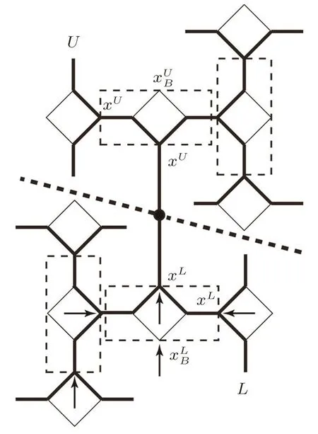
Fig.17 The rede finedunit in SRL for the thermodynamic calculations around the origin.

Similarly,for either xLor xU,recall Eq.(12)and Zm(+)=Bmxm,Zm(?)=Bmymwith Bm=[Zm(+)+Zm(?)],then we have

where SBis the index of the site linked to the bulk tree.With six spins the rectangle unit has 64 possible con figurations thus we can introduce the polynomials:

Then we can obtain the 1-cycle recursive relation:

And the fi x-point solution is the 1-cycle solution xLor xU,Although the actual solution site by site on the surface could be either 1-cycle or 2-cycle.It is important to clarify that the solution xLor xUare exactly the same to the solutions we achieved on the surface in Subsec.2.3(ii).The reason we re-select the basic unit is to obtain a simple polynomial Q for the calculation.

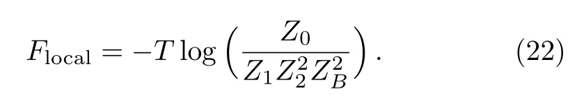
Now we may rewrite Eq.(22)with=0

This local region contains 14 sites,thus the averaged free energy on each site is F=(1/14)Flocal.

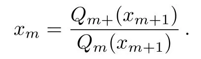
With Eqs.(20)and(21)we can easily obtain the energy density and entropy.A reference thermal behaviors of 1-cycle and 2-cycle solution of SRL with thickness=19,neighbor interaction J=?1,=?1 and all other parameters to be zero are shown in Fig.18.An interesting phenomenon can be observed here:The free energy of 2-cycle solution(crystal state)is higher than the free energy of metastable state between T=1.65 to 2.2,which is abnormal comparing to the bulk behavior in Fig.14.The cross point of 1 and 2-cycle’s free energy at lower temperature can be determined as the melting transition.Above Tm,it presents that the anti-aligned spins arrangement is less stable than the 0.5 solution.The reason of this behavior is yet clear whether it is simply unphysical or it implies a “super-heated crystal” state on the surface.[49]

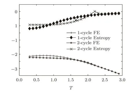
Fig.18 The thermodynamic behaviors of 1-cycle and 2-cycle solution of SRL with thickness=19,J=?1,=?1 and all other parameters to be zero.The black arrow on the entropy show the melting transition at the cross point of free energies(T=1.65),where the entropy of 1-cycle solution will step to 2-cycle solution’s entropy as a first order transition.The ideal glass transition temperature TKcan be clearly observed by the negative entropy of 1-cycle solution.

Below Tmthe behavior is similar to the bulk system.The 2-cycle solution represents the crystal state with a lower free energy and continues to decrease to the free energy of ideal crystal.While the free energy of 1-cycle solution,the metastable state,will reach a minimum point than bind back,this unphysical behavior implies the ideal glass transition.

4 Results and Discussion

4.1 Discussion on Solutions

As introduced above,the thermodynamic calculations are mainly based on the solutions x,i.e.the ratio of PPFs on SRL.A typical 2-cycle solutions of SRL with J and=?1,other parameters as 0,and thickness=16 are shown in Fig.19.

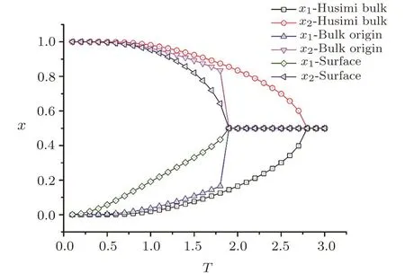
Fig.19 The 2-cycle solutions of SRL with J and J=?1,other parameters as 0,and thickness=16.

The solutions of bulk Husimi lattice are also included for comparison.With the temperature increase,the solutions on surface converge to 0.5 at lower temperature than the Husimi bulk.This indicates a lower melting transition temperature on the surface,which is easy to understand with smaller coordination number and less interactions on the surface,spins on the surface are easier to be anti-aligned with less energy.Also,unlike the symmetrical solutions we usually have,the 2-cycle solution on the surface is asymmetric,because of the hybrid structure on the surface,which de fi nes two different circumstances on the surface square unit and single bond unit respectively.Naturally the spins on the surface square unit have the solution closer to the bulk solution,while the spins on the single bond unit have a less stable solution(closer to 0.5)due to the lower dimension.Depending on the initial seeds adopted for surface calculation,we may also have the other set of surface solutions symmetric to the one in Fig.19.

The 2-cycle bulk solutionsare the solutions at the bulk origin(Fig.12).Since the Husimi lattice plays the bulk portion in SRL,we can expect the bulk origin solution to be identical to the solutions of Husimi lattice if the thickness is large enough to ignore the e ff ects from surface onto bulk,and this expectation is con fi rmed in the region T<2.However the 2-cycle bulk solutions di ff er from the Husimi lattice solutions,and converge to 0.5 solution quickly above T=2.Since the bulk solution comes to be almost steady with thickness larger than 19,this di ff erence is not really caused by the surface e ff ect.Our calculation requires a set of initial seeds for the recursive calculation as the procedure described in Fig.12,the bulk calculation takes the surface solution as its initial seed,in this way,once the surface solution reaches 0.5,the initial seeds of 0.5 will immediately a ff ect the recursive calculation inside the bulk and converges the bulk origin solutions to be 0.5.The bulk origin solutions at converging point with different thickness are shown in Fig.20.We can see the convergence occurs with very slight di ff erences no matter how large the thickness is,while theoretically we should have the bulk origin solutions to be identical with Husimi bulk solutions.Simple to say,because of the property of recursive calculation,the bulk origin solution will be lead away from the exact description by the e ff ect of surface solution in the temperature region between surface melting and Husimi bulk melting transition temperatures,which is not really the “surface e ff ect” in nature.

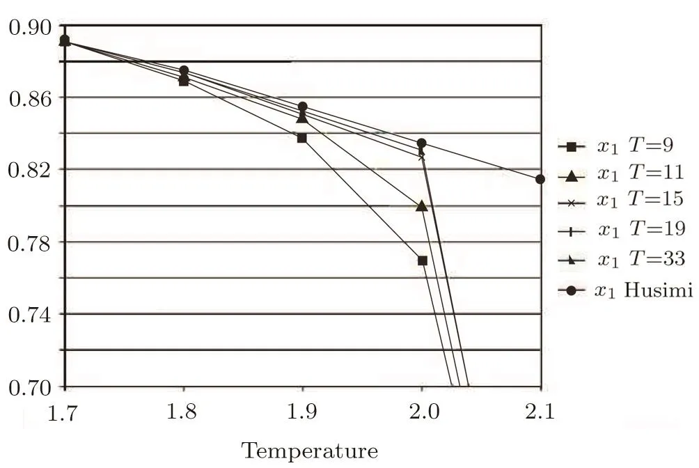
Fig.20 The bulk origin solutions(upper branch)at converging point with different thickness.The curves of thickness=19 and 33 almost overlap and cannot be distinguished in the graph.

This is also one reason we are not interested in calculating the thermodynamics of the whole SRL.There are three facts make this calculation unreliable.Firstly,as mentioned above,in the temperature region between surface melting and Husimi bulk melting transition,the bulk origin solution is a ff ected by the seeds of 0.5 solutions on the surface.Secondly,the recursive calculation technique requires several steps to reach the fi x-point solutions.This implies the calculations on the first few layers closing to the surface are numerical instead of exact calculation.Although for large thickness bulk this error can be neglected,the thermal behaviors associated with exact each different layer is not useful.Thirdly,the recursive structure of SRL proportionally generates more surfaces with increasing thickness.Unlike the regular lattice,in which the contribution of surface can be neglected with a sufficient large bulk,the SRL will have half sites on the surface with in fi nitely large bulk trees.In this way,the thermodynamics on each site is just the averaged value of surface and bulk values.In another word,our approach of SRL is good to track the thermal behaviors on the surface with the account of bulk contributions,but not to discover the thermal behaviors change with various thicknesses.

4.2 The Transition Temperatures Reduction

Our calculations clearly indicate the reduction of both melting and ideal glass transitions temperature on the surface.Figure 21 shows the free energy comparison of Husimi bulk system and SRL.The melting and ideal glass transition temperature are dramatically decreased in SRL comparing to Husimi bulk.In the introduction we have introduced the empirical equation to describe the temperature reduction with the change of the thickness.Since the thickness dependence of transition temperature reduction is not available in our method,and our calculations focus on the transitions right on the surface,we may compare our results to the ratio of glass transition temperatures of bulk and the thinnest free-standing fi lm in others’works,either experimental or simulation results.

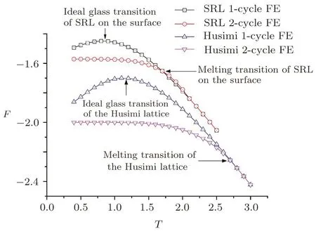
Fig.21 The free energy comparison of Husimi bulk system and SRL.

The TKreduction ratio of SRL is 0.89/1.1=0.809.In Forrest and co-workers’work,the Tgof the thinnest PS fi lm they made is 300 K and the Tgof bulk PS is 369 K,the reduction ratio is 0.813.[11]In Torres and co-workers’MD simulation,this reduction ratio of a free standing fi lm is 0.24/0.3=0.8.[13]In de Pablo and co-workers’MC simulation,this ratio is 0.85/1.08=0.79.[24]

The above SRL result is from the reference model,which is very simple without any particular arti ficial parameters setup,the fact that our ratios are close to others’results may only verify the validity or practice of our method.To particularly describe a real system,the setup of energy parameters is the most critical issue.The effects of energy parameters in our model will be discussed in later section.The fact that similar reduction can be observed in our small molecules model implies that the lower transition temperature on surface/thin fi lm basically originates from the dimension reduction and less interaction constraints.The chain-structure of polymer system may not be the main reason for transition temperature reduction,although it does play important roles to a ff ect the transition properties.

4.3 The E ff ects of Energy Parameters

In this section we are going to study the e ff ects of different energy parameters in SRL by the variation of one parameter with other parameters fixed.The thickness is always set to be 19 for providing a sufficient tree size with relatively short calculation time.

In Eq.(6)we speci fi ed the diagonal interaction energy parameter on the surface to be,di ff ered from the diagonal interaction Jpinside the bulk.And similarly we haveThis speci fication is to enable us setup different interaction circumstance on the surface and provide more versatility in our model.However the e ff ects of either Jpor its counterpart on the surfaceare the same.Thus in this section we are going to simplify the case and setup Jpand,J′′andto be the same.Nevertheless,a variation with fixedwill be discussed in details,because the nearest-neighbor interaction J andhave a much larger weight in the Hamiltonian and play more critical roles in the system.The di ff erence setup of J andprovides the simulation of surface tension,which is critical to the surface properties.

(i)The Diagonal Interaction Jp

In the Hamiltonian Eq.(2),the nearest-neighbor interaction J is negative by the Definition of anti-ferromagnetic Ising model,the system prefers an anti-aligned spins arrangement to obtain a lower energy with a negative first term,then we can also observe that for an anti-aligned spins arrangement,the diagonal spins pairs are in the same state.Therefore,unlike the nearest-neighbor interaction J,a positive diagonal interaction will make the second term to be negative,which encourages the alternating arrangement and increases the transition temperatures(i.e.the crystal is more stable to melt).On the other hand,a negative Jpwill compete with J and trend to destroy the ordered state,which decreases the transition temperature.Because we have four nearest-neighbor and two diagonal interactions in a square unit,the nearest-neighbor interaction outweigh the diagonal interaction.Also,there is no diagonal interaction in the surface single bond unit,which also lowers the contribution of Jp.The variation of Jpwill only moderately change the transition temperatures on the surface;the overall thermal behaviors are similar to the reference case.The thermal behaviors with four different Jpvalues±0.2 and±0.4 are calculated and the melting and ideal glass transition change with Jpvariation is summarized in Table 1.It is obvious that positive Jpwill make the system more stable and increase the transition temperatures,or vice versa.We also found that Jpcannot be larger than±0.5 otherwise stable solutions can not be reached.

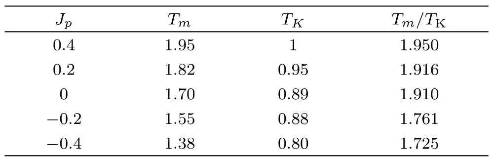
Table 1 The transition temperature variations with different Jp._________________________________________

(ii)The Quadruplet Interaction J′′

Transition temperatures of quadruplet interaction J′′= ±0.2,±0.4,±0.6,±0.8,and ±1.0 with other parameters fixed to be 0 are summarized in Table 2.It is observed that the parameter J′′has a similar e ff ect to Jp:positive J′′will make the system more stable and increase both transition temperatures,and vice versa.We also found that,unlike the limited value of Jp,J′′can be assigned with large value such as±1.0 without destroying the stable solutions.

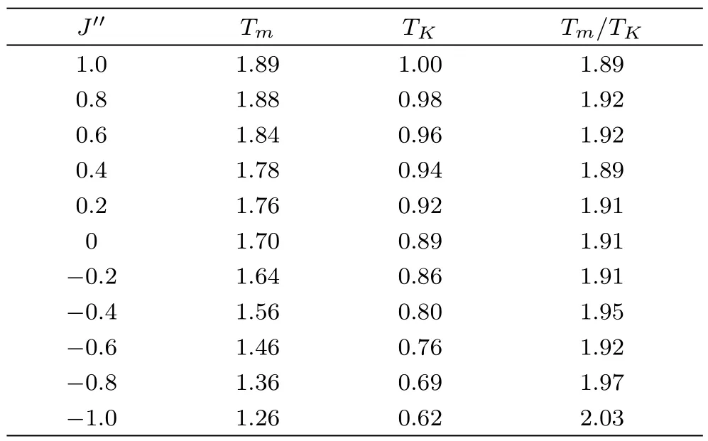
Table 2 The transition temperature variations with J ′′.

One important di ff erence between the e ff ects of Jpand J′′can be observed in Tables 1 and 2:Although both parameters act similarly in changing the transition temperatures,with J′′variation the ratio of Tm/TKis relatively constant unless J′′is assigned with extraordinary values like±1.0,while with the variation of Jpthe ratio of Tm/TKalso changes dramatically.

(iii)The Surface Nearest-Neighbor Interaction

For convenience we setup the energy parameters in the bulk and on the surface,e.g.Jpandto be identical.Nevertheless,the asymmetric interactions and surface tension are the main reason behind the featured properties of surface.Therefore with a fixed bong length,we have to somehow modify the surface interaction to mimic the surface tension or asymmetric interactions.This can be made possible with different J andsetup.With a fixed J=?1,the transition temperatures with variation of=?0.5,?0.7,?0.9,?1.1?1.3 are summarized in Table 3.We can conclude that larger absolute value of negativemakes the system more stable and increases both Tmand ideal Tg.The variation ofrevealed that the surface is more stable with larger tension(?＞?J),or easier to undergo transitions than in the bulk with smaller surface tension(?

Table 3 The transition temperature variations with.

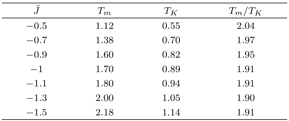
Table 3 The transition temperature variations with.

_______________________________________________________TmTK_Tm/TK?0.51.120.552.04?0.71.380.701.97?0.91.600.821.95?11.700.891.91?1.11.800.941.91?1.32.001.051.90____?1.5______________________________________________________2.181.14_1.91

(iv)The Triplet Interaction J′and Magnetic Field H

With magnetic field H=0,the system has no bias on either+or?spins on a particular site.If a non-zero value of magnetic field H exists,we can expect the 1-cycle solution o ffthe central 0.5 line or asymmetric 2-cycle solutions.A positive H will prefer more+spins and moves the 1-cycle solution higher than 0.5,or vice versa.In our previous research on bulk Husimi lattice,the three spins interaction(triplet)J′acts similarly to magnetic field H in changing the bias of spins.However,in SRL the J′and magnetic field H are not useful,although for a general presentation we still have them in our lattice model and energy equations.The reason is that,the uneven property of the surface on SRL determines the 1-cycle solution can only be 0.5.If a non-zero magnetic field H or triplet interaction J′presents,the 1-cycle solution on the surface cannot be achieved.The single bond unit does not have triple interaction J′and the e ff ect of H is much smaller than it is in the square unit,therefore the anti-aligning property of the single bond will always prefer to have different spins on the other end.In another word,if a 1-cycle solution can be achieved on the single surface bond,it must be the 0.5 solution.Even we can still calculate the thermodynamics of 2-cycle solution on the surface,we must have the corresponding 1-cycle solution to determine the melting and ideal glass transitions.Therefore,we have to abandon the variation of H and J′,which is a disadvantage of the SRL.

5 Conclusion

We construct an inhomogeneous recursive lattice to investigate the thermodynamics and ideal glass transition on the surface/thin fi lm of antiferromagnetic Ising spin system.The model is designed to describe a regular fi nite size square lattice,with a 2D bulk surrounded by 1D surfaces.The fi nite-sized Husimi lattice,which is integrated by 2D square units,are incorporated to represent the bulk part,and single bonds are adopted to represent the surface surrounding the bulk.The lattice is believed to be a reliable approximation to the regular square lattice in the aspect of coordination numbers,i.e.the number of neighbor sites is 4 inside the bulk and 3 on the surface.

The antiferromagnetic Ising model is calculated on the SRL,to capture the order-disorder and ideal glass transition(Kauzmann paradox)by the PFF method and Gujrati trick.Two kinds of stable solutions are achieved by recursive calculation:One is in 2-cycle form and represents the ordered state,the other is in 1-cycle form representing the amorphous/metastable state.The thermal behaviors derived from solutions indicate the melting transition by the cross point of free energies of two solutions,and the ideal glass transition by the negative entropy of 1-cycle solution.Our results agree with others’work that the transition temperatures are dramatically reduced on the surface/thin fi lm comparing which in the bulk.Furthermore,our work shows that,regardless of speci fic properties of particular materials,either polymer or small molecules,this transition temperature reduction can be simply due to the dimension downgrade and lower interaction energy on the surface.

The e ff ects of different energy parameters other than nearest-neighbor interaction such as the diagonal and four spins(quadruplet)interaction are investigated.The variation of energy parameter could either increase or decrease the stability of system and change the transition temperatures according to the Hamiltonian.

While our finding agrees well with others’experimental and simulation results,comparing to previous works,there are two advantages in our approach:(i)In this work our model focuses on the small molecules system,it reveals the fundamental dimensional origin of transition temperatures reduction without involving the long chain properties of polymeric system;(ii)The thermodynamics of systems are derived by exact calculation method,the computation time is much shorter than typical simulation methods,usually the calculation of one set of parameters in the interesting temperature region can be done in less than 100 seconds.

References

[1]M.D.Ediger and J.A.Forrest,Macromolecules 47(2014)471.

[2]J.L.Keddie,R.A.L.Jones,and R.A.Cory,Europhys.Lett.27(1994)59.

[3]S.Kawana and R.A.L.Jones,Phys.Rev.E 63(2001)021501.

[4]J.H.Kim,J.Jang,and W.C.Zin,Langmuir 16(2000)4064.

[5]G.B.DeMaggio,W.E.Frieze,D.W.Gidley,etal.,Phys.Rev.Lett.78(1997)1524.

[6]K.Fukao and Y.Miyamoto,Europhys.Lett.46(1999)649.

[7]J.A.Forrest and J.Mattsson,Phys.Rev.E 61(2000)53.

[8]J.H.van Zanten,W.E.Wallace,and W.L.Wu,Phys.Rev.E 53(1996)R2053.

[9]J.A.Forrest,K.Dalnoki-Veress,J.R.Stevens,and J.R.Dutcher,Phys.Rev.Lett.77(1996)2002.

[10]J.A.Forrest,K.Dalnoki-Veress,and J.R.Dutcher,Phys.Rev.E 56(1997)5705.

[11]J.A.Forrest,K.Dalnoki-Veress,and J.R.Dutcher,Phys.Rev.E 58(1998)6109.

[12]H.Morita,K.Tanaka,T.Kajiyama,T.Nishi,and M.Doi,Macromolecules 39(2006)6233.

[13]J.A.Torres,P.F.Nealey,and J.J.de Pablo,Phys.Rev.Lett.85(2000)3221.

[14]P.Doruker and W.L.Mattice,Macromolecules 31(1998)1418.

[15]G.Xu and W.L.Mattice,J.Chem.Phys.118(2003)5241.

[16]J.Baschnagel and F.Varnik,J.Phys.:Condens.Matter.17(2005)R851.

[17]P.Scheidler,W.Kob,and K.Binder,Europhys.Lett.59(2002)701.

[18]P.Scheidler,W.Kob,and K.Binder,J.Phys.Chem.B 108(2004)6673.

[19]G.D.Smith,D.Bedrov,and O.Borodin,Phys.Rev.Lett.90(2003)226103.

[20]F.Varnik,J.Baschnagel,and K.Binder,Phys.Rev.E 65(2002)021507.

[21]F.Varnik,J.Baschnagel,and K.Binder,Euro.Phys.J.E 8(2002)175.

[22]F.Varnik,J.Baschnagel,K.Binder,and M.Mareschal,Eur.Phys.J.E 12(2003)167.

[23]C.Bennemann,W.Paul,K.Binder,and B.D¨unweg,Phys.Rev.E 57(1998)843.

[24]T.S.Jain and J.J.de Pablo,Macromolecules 35(2002)2167.

[25]K.Huang,Statistical Mechanics,2nd ed.John Wiley&Sons Inc.,New York(1987).

[26]D.Sherrington and S.Kirkpatrick,Phys.Rev.Lett.35(1975)1782.

[27]G.H.Fredrickson and H.C.Andersen,Phys.Rev.Lett.53(1984)1244.

[28]P.D.Gujrati,Phys.Rev.Lett.74(1995)809.

[29]F.Semerianov and P.D.Gujrati,Phys.Rev.E 72(2005)011102.

[30]R.A.Zara and M.Pretti,J.Chem.Phys.127(2007)184902.

[31]T.Yokota,Physica A 379(2007)534.

[32]A.Lage-Castellanos and R.Mulet,Eur.Phys.J.B 65(2008)117.

[33]S.Davatolhagh,D.Dariush,and L.Separdar,Phys.Rev.E 81(2010)031501.

[34]D.Larson,H.G.Katzgraber,M.A.Moore,and A.P.Young,Phys.Rev.B 81(2010)064415.

[35]R.Huang and P.D.Gujrati,Commun.Theor.Phys.64(2015)345.

[36]E.Jurˇciˇsinov and M.Jurˇciˇsin,J.Stat.Phys.147(2012)1077.

[37]R.Huang and C.Chen,Commun.Theor.Phys.62(2014)749.

[38]R.Huang and C.Chen,J.Phys.Soc.Jpn.83(2014)123002.

[39]P.D.Gujrati and M.Chhajer,J.Chem.Phys.106(1997)5599.

[40]M.Chhajer and P.D.Gujrati,J.Chem.Phys.106(1997)8101.

[41]M.Chhajer and P.D.Gujrati,J.Chem.Phys.106(1997)9799.

[42]M.Chhajer and P.D.Gujrati,J.Chem.Phys.109(1998)11018.

[43]M.Chhajer and P.D.Gujrati,J.Chem.Phys.115(2001)4890.

[44]L.Onsager,Phys.Rev.65(1944)117.

[45]B.M.McCoy and T.T.Wu,The Two-Dimensional Ising Model,Harvard University Press,San Diego(1973).

[46]M.Ohzeki,Phys.Rev.E 87(2013)012137.

[47]P.D.Gujrati and A.Corsi,Phys.Rev.Lett.87(2001)025701.

[48]P.D.Gujrati,S.S.Rane,and A.Corsi,Phys.Rev.E 67(2003)052501.

[49]A reasonable guess on this phenomenon is due to the asymmetrical feature of surface:with the as-known Tmdi ff erence between 2D and 3D systems,in a heating process while the surface is already melt above its Tm,the bulk beneath is still in stable crystal form o ff ers considerable constrains to the surface to main its periodic arrangements,i.e.a “superheated crystal”.Further quanti fi ed investigations are in progress to certify this hypothesis.