Changes in Stratospheric ClO and HCl Concentrations Under Different Greenhouse Gas Emission Scenarios

TANG Xiaonan(唐笑男),LIU Yu(劉煜),WANG Weiguo(王衛(wèi)國), SONG Liuming(宋劉明),and LI Weiliang(李維亮)

1 Chinese Academy of Meteorological Sciences,Beijing 100081

2 Department of Atmospheric Sciences,Yunnan University,Kunming 650091

3 Jiaxing Weather Bureau of Zhejiang Province,Jiaxing 314000

Changes in Stratospheric ClO and HCl Concentrations Under Different Greenhouse Gas Emission Scenarios

TANG Xiaonan1,2(唐笑男),LIU Yu1?(劉煜),WANG Weiguo2(王衛(wèi)國), SONG Liuming3(宋劉明),and LI Weiliang1(李維亮)

1 Chinese Academy of Meteorological Sciences,Beijing 100081

2 Department of Atmospheric Sciences,Yunnan University,Kunming 650091

3 Jiaxing Weather Bureau of Zhejiang Province,Jiaxing 314000

In this study,comparison of model results and satellite observations reveals that the Whole-Atmosphere Community Climate Model(WACCM-3)reasonably well reproduced the distributions and seasonal variations of ClO and HCl concentrations.In three greenhouse gas emission scenarios(A1B,A2,and B1), the ClO,Cl,ClONO2,and HCl concentrations would gradually decrease with time as emissions of ozone depleting substances(ODS)steadily decrease.The rates of the changes in the ClO,Cl,ClONO2,and HCl concentrations are different in the same emission scenario and the rates of change in the same composition concentration are different for different emission scenarios.The ClO,Cl,and ClONO2concentrations decrease fastest in scenario A2,next fastest in scenario A1B,and slowest in scenario B1.In contrast,the HCl concentration decreases fastest in scenario B1.The ozone concentration recovers quickly,and is highest in scenario A2.The results show that a rapid decrease in the ClO concentration is an important reason for the accelerated recovery of the ozone layer in scenario A2.

ozone,ClO,HCl,change,trend,greenhouse gas emission scenario

1.Introduction

Ozone is found in trace concentrations in the atmosphere.About 90%of the ozone in the atmosphere is in the stratosphere and about 10%is in the troposphere(Wang et al.,2001).In the absence of any interference from externalfactors,there is a naturalbalance between the chemicalprocesses that produce and destroy ozone in the stratosphere(Liu et al.,1999). Increasing anthropogenic emissions of ozone-depleting substances(ODSs)since the 1970s,such as chlorineand bromine-containing hydrocarbon compounds and nitrogen oxides,caused the abundance of ozone in the stratosphere to decrease markedly between the 1970s and 1990s.The ozone concentrations in Antarctica in the springs between 2006 and 2009 were about 40%lower than in 1980,and the average total ozone concentration remained roughly 2.5%lower than the 1964-1980 average between 60°S and 60°N(WMO, 2010).

Molina et al.(1974)proposed a mechanism for the depletion ofozone by chlorofluorocarbons.Farman et al.(1985)discovered that stratospheric ozone concentrations over Antarctica decreased rapidly and significantly in the spring and gradually recovered later in the year;this phenomenon became known as the Antarctic“ozone hole”.The Antarctic ozone hole has tended to become more severe since it was discovered.The discovery of the Antarctic ozone hole helped us to understand the importance of protecting the ozone layer.The international community adopted the Montreal Protocol for protecting the ozone layer in 1987,and some amendments and adjustments were made later.The implementation of the protocol and its amendments and adjustments have led to global ODS production and consumption being curbed successfully.The abundances of chlorine-and brominecontaining substances that are formed through the degradation of ODSs are decreasing in the troposphere,and the totalabundance of chlorine in the troposphere had decreased to 3.4 parts per billion(ppb) by 2008 from a peak of 3.7 ppb(WMO,2010).

Lower abundances of ODSs will lead to increasing of ozone concentrations in the stratosphere,and this is a major factor that contributes to the ozone layer recovering.Several factors other than ODSs also affect the future evolution of ozone in the stratosphere. These include changes in(1)the temperature and circulation of the stratosphere caused by changes in the abundances of long-lived greenhouse gases(GHGs), (2)stratospheric aerosol abundances,and(3)abundances of highly reactive stratospheric hydrogen-and nitrogen-containing compound gases that are from sources emission,such as methane(CH4)and nitrous oxide(N2O).These factors can interfere with the effects of ODSs on stratospheric ozone(WMO,2010).

Finding a way of projecting future ozone abundances based on an understanding of the complex linkages between ozone and climate change is an important scientific challenge.The most recent simulation results are summarized in the 2010“Ozone Assessment Report”.The A1B GHG and A1 ODS emission scenarios are predicted to lead to the global annually averaged total ozone abundance returning to the 1980 levels before the mid-21st century,which is earlier than when ODS abundances will return to the 1980 levels. This is because ozone will be destroyed more slowly with the presence of GHGs causing the upper stratosphere to cool(WMO,2010).

In addition to the recovery of the ozone layer, a key concern is how ODS abundances will change, because ODS abundances are directly related to the recovery of the ozone layer.Chlorine and bromine atoms released during the degradation of ODSs in the stratosphere can form inorganic chlorine-and bromine-containing compounds.These compounds are called totalinorganic chlorine(Cly)and totalinorganic bromine(Bry).The combination of Clyand Bryamounts in the stratosphere represents the potential for the ozone to be destroyed by halogen-containing compounds.This combination is defined as the equivalent stratospheric chlorine(ESC),which can be used to approximately represent the ODS abundance.Simulation results have indicated that the stratospheric abundances of ODSs will return to the 1980 levels around 2045-2060(WMO,2010).The ESC can represent changes in the total halogenated substance abundances well,so it has been used in many studies on the changes of ODS abundances.

It is well known that ClOxis the key Clyspecies that destroys ozone(Molina et al.,1974).Chlorine nitrate(ClONO2)and hydrogen chloride(HCl)are the main Clyreservoir species.Therefore,a change in the ESC will not reflect changes in the abundances ofdifferent Clyconstituents that affect ozone recovery. Very few studies have been performed on this subject. In this work,we will explore the changes in the abundances of different Clyconstituents as the ozone layer recovers under different GHG emission scenarios,with the purpose of attempting to better understand the impacts of GHGemissions on the recovery ofthe ozone layer.

2.Models and data

2.1 Model description

The Whole-Atmosphere Community Climate Model(WACCM-3)was used to simulate the ozone recovery and the changes in Clyconstituent abundances under the GHG emission scenarios B1,A1B, and A2,and the ODS emission scenario Ab.WACCM-3 is a three-dimensionalglobalatmosphere model that was recently developed by NCAR of US.WACCM-3 is an extension of the Community Atmosphere Model (CAM-3),thus it has 66 vertical levels extending from the earth’s surface to the thermosphere,reaching ageometric altitude of 140 km.The model uses a finite volume dynamic framework(Lin,2004)and a finitevolume dynamic core.WACCM-3 contains all of the physical processes that were included in CAM-3,with some improvements in the gravity wave drag and vertical diffusion schemes.

Several physics and chemistry modules have been added to WACCM-3,and the photochemical“Model for Ozone and Related Chemical Tracers”module MOZART-3 has been incorporated and expanded to trace 57 chemical substances,72 photochemical reactions,and 149 gas-phase reactions(Kinnison et al., 2007).WACCM-3 takes into account more processes than does CAM-3,and these include shortwave heating and photolysis from the Lyman-alpha to far ultraviolet radiation,and molecular diffusion and diffusive separation.The parameterizations ofgravity wave breaking and diffusion in the middle and upper atmospheres are included,and the effects of longwave radiation above 60 km with non-local thermodynamic equilibrium(for which atomic excitation,ionization,and radiation cannot be described by only using the local temperature)are parameterized(Sassi et al.,2002).

2.2 Emission scenarios

The“Special Report on Emissions Scenarios”, published by the Intergovernmental Panel on Climate Change(IPCC)in 2000,contains scenarios for future changes in GHG emissions,which have been widely used to project future climate change.We used the A1B,B1,and A2 emission scenarios described in the IPCC 3rd Assessment Report(AR3).The A1 scenario family describes a future world in which the regions develop and converge into three groups that are distinguished from each other by their technological emphases on energy systems,called A1F1,A1B,and A1T.The A1B scenario used in our work has all energy sources that are used in balance.In this scenario, the CO2-based annualGHGemission rate continues to grow from 2000 to 2060 and then drops after 2060,and the CO2concentration in the atmosphere continues to increase throughout the 21st century.The B1 scenario is a more harmonious world that uses more ecologically benign systems than those used in the other scenarios.In the B1 scenario,the CO2-based annual GHG emission rate increases until 2050 and decreases after 2050,and the CO2concentration increases until 2090 and then remains constant.The A2 scenario is for a more divided world in which the CO2-based annual GHG emission rate increases constantly,at a higher rate than in the A1B and B1 scenarios,and the CO2concentration also increases constantly.

Implementing the Montreal Protocol and its amendments and adjustments has led to the production and consumption of ODSs decreasing and the ODS concentrations in the atmosphere decreasing. The World Meteorological Organization(WMO,1998) described future ODS emission scenarios A,B,C,and E,which were based on the relevant conventions and protocols.Of these scenarios,the Ab scenario was the best-designed estimate,and it was based on the production and consumption trends for the time when the scenarios were developed(WMO,2002).

2.3 Scenario tests

The 1951-2001 sea ice and sea surface temperature data were taken from the UK Met Office Hadley Centre monthly sea ice and sea surface temperature dataset(HadISST),and they were used with the A1B emission scenario to run a continuous integration from 1951 to 2001.Then,with data for January 2001 as the initial field,a continuous integration was run for 99 yr, from 2001 to 2099,using the emission source data from the A1B,A2,and B1 GHG emission scenarios.The sea ice and sea surface temperature simulation results from a coupled air-sea model(the Community Earth System Model)for the three scenarios were then used to give the A1B,A2,and B1 emission scenario tests that are used in this paper.

2.4 Data

We employed satellite observations of ClO and HCl abundances to validate the ability of the model to simulate changes in the abundances of different Clyconstituents.The Aura satellite,which was launched on 15 July 2004 as the third major component of the Earth Observing System,carries a microwave limb sounder(MLS)to observe the abundances of O3,HCl, HNO3,ClO,N2O,and other species in the stratosphere at latitudes of 82°S-82°N at different effectivevertical height ranges for different species(100-0.02 hPa for O3,100-0.32 hPa for HCl,215-1.5 hPa for HNO3,147-1 hPa for ClO,and 100-0.46 hPa for N2O). The MLS data(version 3.3)were used in this study. These data were converted into three-dimensionalgrid data with a horizontalresolution of1.875°latitude and 2.5°longitude by using the filter criteria for different species for 2005-2012.Santee et al.(2008)evaluated the MLS(version 3.3)ClO data and found that clouds affected the accuracy of the ClO observations,especially below 100 hPa.A vertical range of 100-1 hPa was used for ClO in our study,and a cloud effect filter was used even though the probability of clouds being present was less than 3%.

3.Comparison of simulation results with observations

We compared the satellite data with the simulation results to assess the ability of the model in simulating the abundances of different Clyspecies.The 2005-2012 averaged satellite ClO observations and the simulation results for the same period under the A1B emission scenario are shown in Fig.1.As can be seen, there were two centers with high ClO concentrations in the upper stratosphere,one at high latitude in the Southern Hemisphere and the other at high latitude of the Northern Hemisphere.The locations of these high centers were different in different seasons,but both areas varied in similar ways.Each of the high centers was in the polar region in spring and summer and at a high latitude in autumn and winter,and the height of each center was about 1-3 hPa.There was one center of high ClO concentrations in the lower stratosphere at high latitudes and in the polar region in the Southern Hemisphere in winter and spring.There was one center of high ClO concentrations in the lower stratosphere at high latitudes in the Northern Hemisphere in winter.As can be seen from Fig.1,the model accurately reproduced the spatial distribution of ClO in the stratosphere.Two high centers in the upper stratosphere were captured,one at high latitudes in each of the hemispheres.One area of high ClO concentrations in the lower stratosphere was displayed,at high latitudes and in the polar region in the Southern Hemisphere.The seasonal variations in the two ClO high concentration centers in the upper stratosphere, i.e.,changes in the concentrations and locations of the centers,were also well simulated.However,the observed and simulated ClO concentrations were significantly different,and ClO high center in the lower stratosphere in the Northern Hemisphere was not reproduced at all.These failures were probably caused by the differences in the sea temperature between simulation results and the observed data,which led to the lower stratospheric temperature in the Arctic beinghigher in the simulation than in the observed data (figure omitted).This may have affected the ability of the model to appropriately simulate the heterogeneous chemical processes and ClO concentrations.

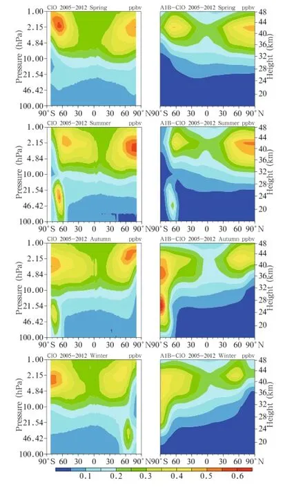
Fig.1.Seasonal variations in the mean ClO abundance from 2005 to 2012.The MLS satellite data are on the left, and the simulation results under the A1B scenario are on the right.

The 2005-2012 averaged satellite HCl observations and the simulation results for the same period under the A1B emission scenario are shown in Fig.2. The HCl vertical distribution features,i.e.,increasing HCl concentration with altitude,can be seen in Fig. 2.At the altitude below 10 hPa,the HCl concentration was higher at higher latitudes than that at lower latitudes,and,except in the Antarctic winter,was approximately symmetrical in the Southern and Northern Hemispheres.The distribution was more even at the altitudes above 10 hPa.Under the A1B emission scenario,the model accurately reproduced the HCl distribution and its seasonal variations,including the emergence of a low center in the Antarctic in winter. However,the simulated HCl concentrations in the upper stratosphere were rather low.In summary,the model decently reproduced the ClO and HCl distributions and seasonal variations as from satellite observations,so the model could be used to study changes of other Clyspecies under different emission scenarios.

Fig.2.As in Fig.1,but for HCl.

4.Analysis of results

4.1 Changes in global column ozone concentrations

It was pointed out in the latest ozone assessment report(WMO,2010)that the total abundances of anthropogenic ODSs in the troposphere peaked between 1992 and 1994 and then decreased,reaching 8%-9% below the peak abundances by 2005.The abundances of ODSs in the stratosphere have continued to follow a relatively shallow downward trend since the peak in the 1990s;this is consistent with surface observations of ODS abundances and the time lag for them to be transported to the stratosphere.Satellite data (Jones et al.,2011)have shown that the HCl abundance in the upper stratosphere(35-45 km)has decreased from a peak in 1997 by 5.1%per decade in the Northern Hemisphere(30°-50°N)and by 5.2%per decade in the Southern Hemisphere(30°-50°S),and that the ClO abundance has decreased from a peak in the 1990s by 7.8%per decade in the equatorial zone (20°S-20°N).These observations illustrate that the recovery in ozone concentrations in the stratosphere in recent years has been related to decreasing ODS concentrations in the stratosphere.

The recovery of the ozone layer in the future,predicted by WACCM-3 under the three GHG emission scenarios and with an assumption that ODS concentrations continue to decrease at the current rate,is shown in Fig.3.It is found that the ozone concentration in the stratosphere will return to the 1980 level around 2035 under the A1B and A2 scenarios.The ozone concentration in the stratosphere willthen reach a concentration in 2060 that will remain stable untilthe end of the century under the A1B scenario,and that after 2035 the ozone concentration in the stratosphere will increase under the A2 scenario.The ozone concentration will recover relatively slowly under the B1 scenario,returning to the 1980 level around 2050 and then increasing more slowly than under the A1B and A2 scenarios.Overall,the simulation results based on the three different GHG emissions scenarios project that the ozone concentration will return to the 1980 level or higher by the middle of the 21st century.The maximum predicted concentration is 4.5%higher than the 1980 levelunder the A2 scenario, 2.46%higher under the A1B scenario,and only 1.31% higher under the B2 scenario(which willgive the slowest recovery).These results are in general consistent with the latest ozone assessment report(WMO,2010).

4.2 Changes in ClOxconcentrations

The recovery of the ozone layer is related to decreasing ODS concentrations,but the ozone concentrations will recover at different rates under different GHG emission scenarios even if the ODS concentrations decrease at the same rate.The results of the present study suggest that there are two reasons for this.The first reason is that the temperature will change in different ways under different GHG emission scenarios because the cooling of the stratosphere will decrease the rate at which ozone is depleted,mainly because of the effects on odd oxygen species(Jonsson et al.,2004).The second reason is that the circulation patterns will change(WMO,2010).We next analyze in detail the changes predicted in the concentrations of several Clyspecies under different GHG emission scenarios to study the factors that could lead to different ozone recovery rates to occur.

We first analyze the changes in ClO concentrations.The spatial distributions of the zonal mean deviations between the 2030s and 2070s under the A1B, A2,and B1 emission scenarios are shown in Fig.4.It can be seen that changes in ClO concentrations have similar distributions under different emission scenarios.There are two areas in which ClO concentrations will decrease in the upper stratosphere:one is located at 60°S and the other at 60°N.It is obvious that the maximum central values decrease,-0.11 ppbv in the Southern Hemisphere and-0.12 ppbv in the Northern Hemisphere,under the A2 scenario.The ClO concentration in the lower stratosphere will decrease more in the Antarctic than in the Northern Hemisphere.From the ClO distribution(Fig.1)and the ClO concentration changes(Fig.4),it is clear that the maximum ClO concentration and the greatest changes will occur at approximately 2 hPa.

The changes in the global mean ClO concentration over time at 2.15-hPa altitude are shown in Fig. 5a,which shows that the ClO concentration will continue to decrease over time,from 0.32 ppb in 2001 to 0.1 ppb in 2100,under the three scenarios,more quickly before than after 2050.It is also seen that the A2 scenario will cause the ClO concentration to decrease fastest and that the A1B scenario will cause the ClO concentration to decrease next fastest.The changes under the A2 and B1 scenarios are compared to the changes under the A1B scenario in Fig.5b, which indicates that the changes in the ClO concentration will be similar under the A2 and A1B scenarios until 2045 but that the concentrations will then decrease more quickly under the A2 scenario until the concentration under the A2 scenario reaches 25% less than the concentration under the A1B scenario in 2100.The ClO concentration will decrease more slowly in the B1 scenario than in the A1B scenario,and the difference in the ClO concentration will increase between 2010 and 2050,reaching a maximum of 10%in 2050,and then becoming progressively smaller.

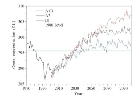
Fig.3.Time series of the globally averaged total column ozone concentrations,as predicted by WACCM-3,under the A1B,A2,and B1 scenarios with an assumption that ODS concentrations continue to decrease.

The spatial distributions of change in the ClO concentration between the A2 and A1B scenarios and between the B1 and A1B scenarios in the 2060s are shown in Fig.6.The spatial distributions of the differences are similar to the ClO spatial distribution under all the scenarios,and the largest differences are predicted to be in the upper stratosphere, with a maximum of 0.012 ppb in midlatitudes of the Southern Hemisphere and the other in midlatitudes of the Northern Hemisphere.Two areas of extreme differences(one positive and the other negative)are predicted to be over the Antarctic,one in the middle stratosphere(30-10 hPa)and the other in the lower stratosphere(100-30 hPa).This change is found to be related to heterogeneous chemical processes in the Antarctic region.These results indicate that there will be clear differences between the ClO concentration changes under the three scenarios,and higher GHG emissions will lead to the ClO concentration decreasing more quickly.

We then analyze the changes in the Clconcentrations.The spatial distributions of the zonal mean deviations between the 2030s and 2070s under the A1B, A2,and B1 emission scenarios are shown in Fig.7. It can be seen that the changes in the Cl concentrations have similar distributions under different emission scenarios.The changes mainly occur in the upper stratosphere,and larger differences appear at higher altitudes.It is clear that the largest decrease(-4.0pptv)will occur in the upper stratosphere under the A2 scenario.The changes in the Clconcentrations are smaller than the changes in the ClO concentrations, and this is because the Cl concentration is lower than the ClO concentration.

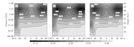
Fig.4.Zonal mean deviations in ClO concentrations(ppbv)between the 2030s and 2070s under the(a)A1B,(b)A2, and(c)B1 scenarios.

Fig.5.(a)Time series of ClO concentrations between 60°S and 60°N at 2.15 hPa under the A1B,A2,and B1 scenarios. (b)Temporal changes in ClO concentrations under the A2 scenario relative to those under the A1B scenario,and under the B1 scenario relative to those under the A1B scenario at 2.15 hPa.

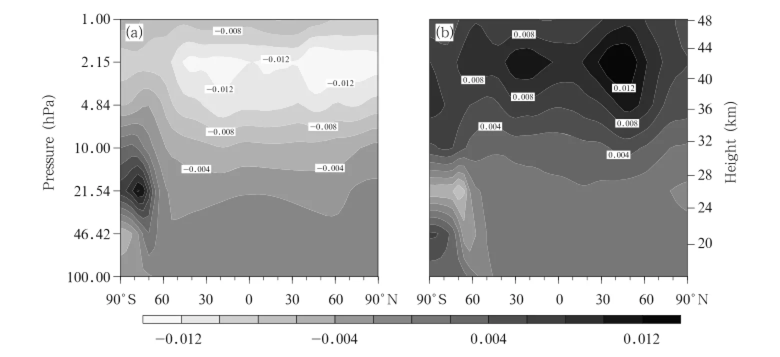
Fig.6.Differences in ClO concentrations(ppbv)between pairs of scenarios in the 2060s.(a)A2 minus A1B and(b) B1 minus A1B.

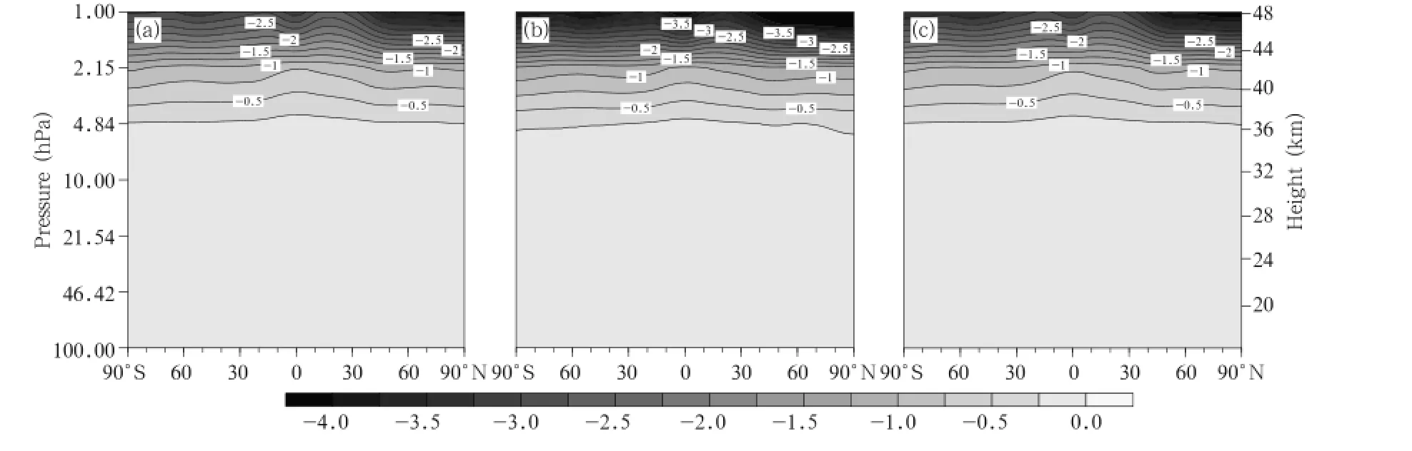
Fig.7.As in Fig.4,but for Cl concentrations(pptv).

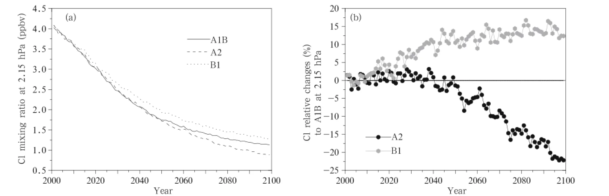
Fig.8.As in Fig.5,but for Cl concentrations(pptv).

The changes in the mean Cl concentration between 60°S and 60°N at 2.15 hPa over time are shown in Fig.8a,which demonstrates that the Cl concentration will continue to decrease over time under all three scenarios,from 4.1 pptv in 2001 to 1.25 pptv in 2100 (similar to the ClO changes),with the rate of change being higher before than after 2050.In addition,thedecrease in Cl concentrations are fastest under the A2 scenario and next fastest under the A1B scenario.The changes under the A2 and B1 scenarios relative to the changes under the A1B scenario are shown in Fig.8b, which shows that the changes in the Cl concentration under the A2 and A1B scenarios are identical before 2045,but the decrease in the Cl concentration would be larger under the A2 scenario than under the A1B scenario after 2045,with the Cl concentration under the A2 scenario being 23%lower than the concentration under the A1B scenario in 2100.The Cl concentration decreases more slowly under the B1 scenario than under the A1B scenario,the concentrations under the A1B scenario will be 10%lower than the concentration under the B1 scenario in 2050.The difference is predicted to increase slowly after 2050,and the concentration under the A1B scenario will be 15%lower than the concentration under the B1 scenario.

The differences in the changes in Cl concentrations between the A2 and A1B scenarios and between the B1 and A1B scenarios in the 2060s are plotted in Fig.9 to allow us to better understand the spatial distributions of the differences in the changes of Cl concentration under the three emission scenarios.The changes are similar under all the scenarios,and the largest differences between different scenarios are in the upper stratosphere(the maximum difference there is 0.6 pptv).These results indicate that there are clear differences between the changes in the Cl concentrations under the three scenarios,and that higher GHG emission scenario will lead to the Cl concentration decreasing more quickly.

4.3 Changes in concentrations of the reservoir compound ClONO2

ClONO2is a product of the reaction between ClO and NO2.It can be converted from a reservoir to an active constituent of Clythrough heterogeneous chemical processes,and it can ultimately affect the ClOxconcentration.Therefore,ClONO2is a very important constituent of Cly.The spatial distributions of the zonal mean deviations in the ClONO2concentration between the 2030s and 2070s under the A1B,A2, and B1 emission scenarios are shown in Fig.10.As can been seen,the changes in the ClONO2concentration possess similar distributions under the different emission scenarios.Two extreme centers of ClONO2concentration decrease in the middle stratosphere are found,one at 45°S and the other at 45°N.It is clear from concentrations of these centers that the maximum values decrease,with-0.25 ppbv appearing under the A2 scenario.

Fig.9.As in Fig.6,but for Cl concentrations(pptv).

From the changes in the ClONO2concentrations, it is clear that the maximum ClONO2changes willoccur approximately at 20-10 hPa.The changes in the mean ClONO2concentration from 60°S to 60°N over time at 10 hPa are shown in Fig.11a.It is seen that the ClONO2concentrations continue to decrease over time under all three scenarios,from 0.32 ppbv in 2001 to 0.1 ppbv in 2100,and more quickly before than after 2050.Moreover,the fastest decrease in the ClONO2concentration occurs under the A2 scenario and thenext fastest under the A1B scenario.The changes under the A2 and B1 scenarios are plotted against the changes under the A1B scenario in Fig.11b,from which it can be seen that the changes in the ClONO2concentration are similar under the A2 and A1B scenarios before 2045,but the ClONO2concentration will change more quickly under the A2 scenario than under the A1B scenario from 2045 to 2100(untilthe ClONO2concentration is 20%lower under the A2 scenario than under the A1B scenario in 2100).The ClONO2concentration will decrease more slowly under the B1 scenario than under the A1B scenario,and the difference between the two will increase between 2010 and 2050, reaching a maximum of 10%in 2050,and then becoming progressively smaller after 2050.

The differences in the changes of ClONO2concentration between the A2 and A1B scenarios and between the B1 and A1B scenarios in the 2060s are plotted in Fig.12.The changes are similar under all scenarios,and the largest differences between different scenarios exist in the middle stratosphere.Two areas with large differences are predicted,one between 30°and 40°S and the other between 30°and 40°N. The maximum difference is 0.036 ppbv.One area with a large difference occurs in the lower stratosphere (10-100 hPa)over the Antarctic(similar to the area predicted for ClO but with the opposite effect),suggesting that the changes are related to the heterogeneous chemical processes in the Antarctic region. These results indicate that there would be clear differences in the changes to occur in the ClONO2concentrations under the three scenarios,and that higher GHG emissions scenario would lead to the ClONO2concentration decreasing more quickly.

4.4 Changes in concentrations of the reservoir compound HCl

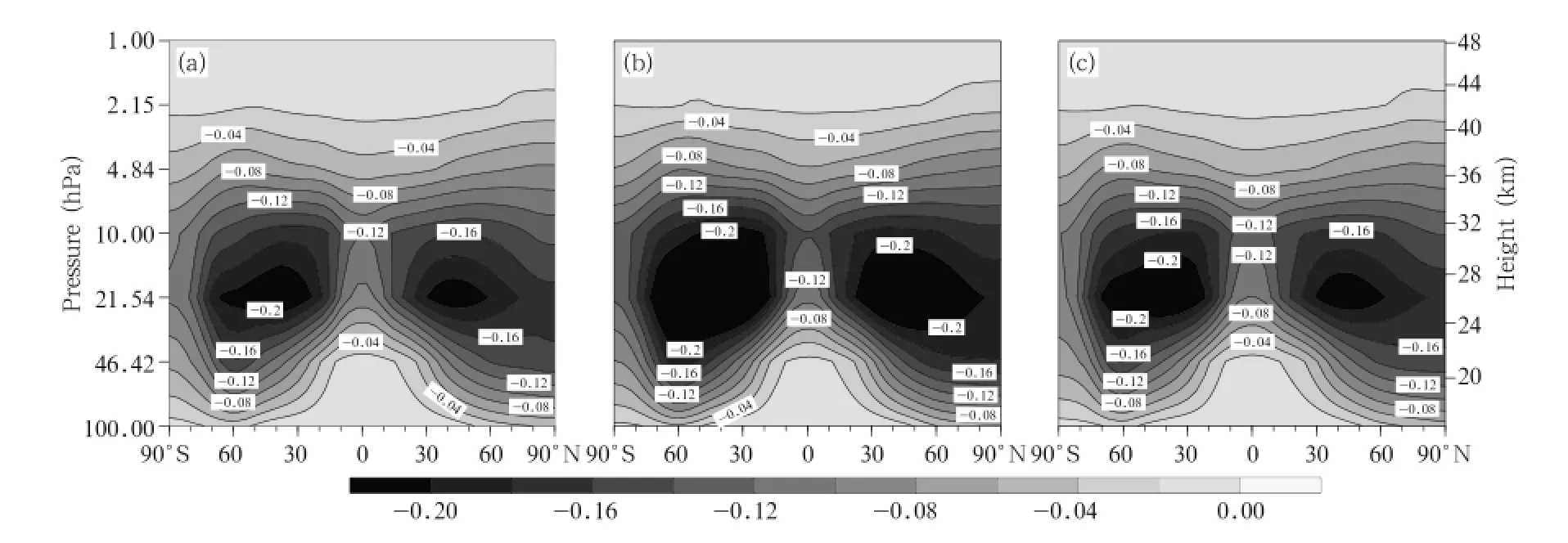
Fig.10.As in Fig.4,but for ClONO2concentrations(ppbv).

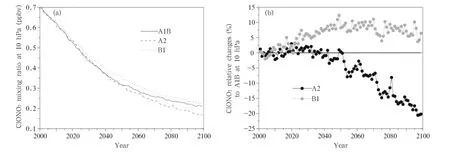
Fig.11.As in Fig.5,but for ClONO2concentrations(ppbv)at 10 hPa.

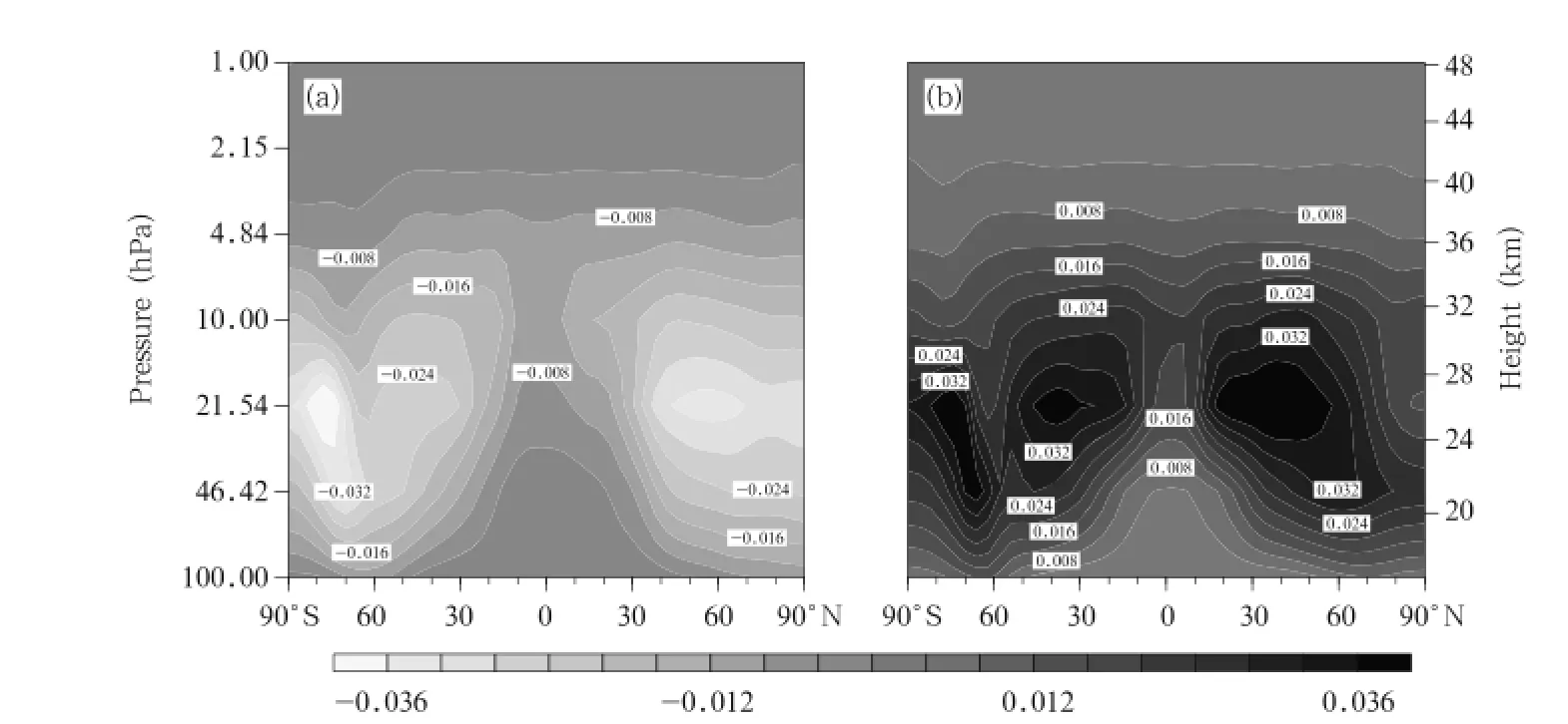
Fig.12.As in Fig.6,but for ClONO2concentrations(ppbv).

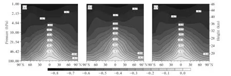
Fig.13.As in Fig.4,but for HCl concentrations(ppbv).

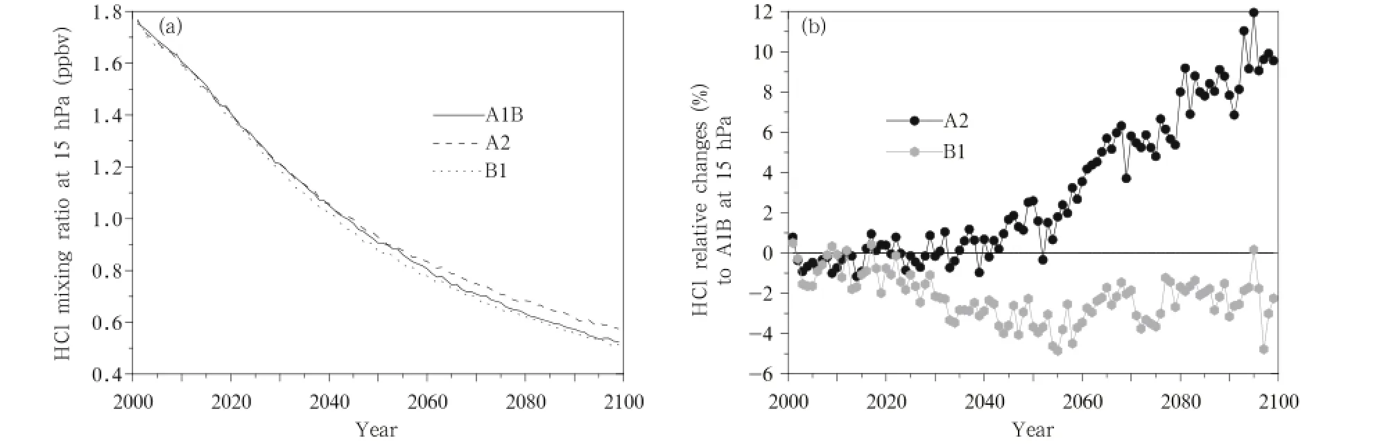
Fig.14.As in Fig.5,but for HCl concentrations(ppbv)at 15 hPa.

HCl is an important reservoir component for the production of Cly.HCl is transported to the troposphere and then removed from the atmosphere by wet deposition,which is the only way the stratospheric Clycan be removed from the atmosphere.The spatial distributions of the zonal mean deviations in HCl concentrations between the 2030s and 2070s under the A1B,A2,and B1 emission scenarios are shown in Fig. 13.As can been seen,the changes in the HCl present similar distributions under the different emission scenarios.The HCl concentration decreases as the altitude increases,but this occurs less in the tropicalareas than in high latitudes,corresponding to the distribution of HCl concentrations.The largest decrease(-0.7 ppbv)occurs under the A2 scenario.The changes in the HCl concentration from 60°S to 60°N over time at 15 hPa are shown in Fig.14a.It is seen that the HClconcentrations continue to decrease over time under all three scenarios,from 1.76 ppbv in 2001 to 0.5 ppbv in 2100,and more quickly before than after 2050.Furthermore,the fastest decrease in the HCl concentration is predicted to occur under the B1 scenario,and the next fastest under the A1B scenario.The changes under the A2 and B1 scenarios are plotted relative to the changes under the A1B scenario in Fig.14b,which indicates that changes in the HCl concentration will be similar to those under the A2 and A1B scenarios before 2045,but the HCl concentration will decrease more slowly under the A2 scenario than under the A1B scenario after 2045(untilthe HClconcentration is 10% larger under the A2 scenario than under the A1B scenario in 2100).The HCl concentration will decrease more quickly under the B1 scenario than under the A1B scenario,and the difference between the two will increase between 2010 and 2050,reaching 5%in 2055, and then becoming progressively smaller after 2055.

The differences in the changes in HCl concentrations between the A2 and A1B scenarios and between the B1 and A1B scenarios in the 2060s are plotted in Fig.15 to allow us to better understand the spatial distribution of the differences in the changes of HCl concentrations under the three emission scenarios.The changes are similar under all the scenarios, and the largest differences between different scenarios are found in the middle stratosphere.Two areas with large differences are predicted,one between 30°and 40°S and the other between 30°and 40°N.The maximum difference is 0.04 ppbv.One area with a large difference occurs in the middle and lower stratosphere(10-100 hPa)over the Antarctic(similar to the area predicted for ClO but with the opposite effect). This indicates that the changes are related to heterogeneous chemical processes in the Antarctic region. Under the B1 scenario,the changes in HCl concentrations in the lower stratosphere in the tropics and the Antarctic are the opposite ofthe changes in the middle and high latitudes.This indicates that there would be clear differences in the changes to occur in HCl concentrations under the three scenarios,and that higher GHG emissions would lead to the HCl concentrations decreasing more slowly.

4.5 Changes in Clscolumn concentrations

The changes in the globalmean totalcolumn concentration of Cls(=ClO+Cl+ClONO2+HCl)over time are shown in Fig.16a.It is seen that the total column Cls concentration will continue to decrease over time under the three scenarios from 12.5 mm(the thickness under standard atmospheric conditions)in 2001 to 4 mm in 2100,with the rate of decrease being higher before than after 2050.In addition,the fastest decrease in the total column Clsconcentration occurs under the A2 scenario and the next fastest under the A1B scenario.The changes under the A2 and B1 scenarios are plotted relative to the changes under the A1B scenario in Fig.16b,from which it can be seen that the changes in the total column Clsconcentration is similar under the A2 and A1B scenarios before 2030,but the Clsconcentration will decrease morequickly under the A2 scenario than under the A1B scenario after 2030(until the Clsconcentration is 4% lower under the A2 scenario than under the A1B scenario in 2100).The total column Clsconcentration will decrease more slowly under the B1 scenario than under the A1B scenario,then the changes under the B1 and A1B scenarios become similar until 2020,and then the changes occur more slowly under the B1 scenario than under the A1B scenario between 2020 and 2100(until the Clsconcentration is 4%larger under the B1 scenario than under the A1B scenario in 2100). The final difference(4%)is,however,relatively small compared with the final differences in the concentrations of the four components(ClO,Cl,ClONO2,and HCl).

Fig.15.As in Fig.6,but for HCl concentrations(ppbv).

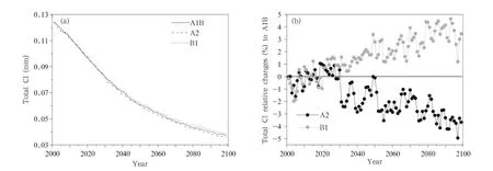
Fig.16.As in Fig.5,but for Clscolumn concentrations in the troposphere and stratosphere.

5.Conclusions and discussion

As can be seen from the results described above, continuously decreasing emissions of ODSs will lead to decreasing concentrations of ClO,Cl,ClONO2,and HCl over time.The changes in the ClO,Cl,ClONO2, and HCl concentrations will be different under the same GHG emission scenario.The rates at which the concentrations of the same species change will be different under different GHG emission scenarios.The ClO,Cl,and ClONO2concentrations decrease faster under the A2 scenario than under the A1B scenario and faster under the A1B scenario than under the B1 scenario.In contrast,the HCl concentrations decrease faster under the B1 scenario than under the A1B scenario and faster under the A1B scenario than under the A2 scenario.The total column Clsconcentration decreases gradually over time,with the changes occurring at slightly different rates under different emission scenarios.The decrease occurs slightly faster under the A2 scenario than under the A1B scenario,and the concentration will be 4%less under the A2 scenario than under the A1B scenario by 2100.This is mainly caused by high concentrations of HCl and the intense Brewer-Dobson circulation(Garcia and Randel,2008) under the A2 scenario,meaning that more HCl would be transported to and cleared from the troposphere than under the A1B scenario.

Jonsson et al.(2004)used a three-dimensional chemistry climate model to study changes in the stratospheric temperature and ozone concentration when the CO2concentration is doubled,and to study the mechanisms involved in changes in the ozone concentrations in different regions.Their results indicated that doubling the CO2concentration would lead to stratospheric cooling by a maximum of 10-12 K and an increase in the ozone concentration by 10%-20%. The ozone concentration would increase at altitudes of 30-70 km mainly because of the negative relationship between the occurrence of the O+O2+M→O3+ M reaction and the temperature.A 10%increase in the reaction coefficient would lead to a 12%increase in the ozone concentration.The ozone concentrations would increase by about 5%at altitudes below 60 km, and there would be a 25%decrease in the reaction coefficient for the O+O3→2O2reaction and a decrease in the NO2concentration.It is also suggested that the ClO concentration would increase by a maximum of10%at altitudes of 30-50 km and decrease in other regions,and that the ClO+O→Cl+O2reaction coefficient would decrease(by around-2%).These results provide the main basis for the effects of GHGs on ozone recovery.However,heterogeneous chemical processes were not taken into consideration in the study just described.

Our model gave different ClO results from the results of Jonsson et al.(2004)because heterogeneous chemical processes were incorporated into our model. The ClO concentration in the stratosphere is predicted to decrease quickly in the high emission scenario,and particularly quick decreasing of ClO concentrations occur at 30-50 km.These decreased ClO concentrations may be caused by heterogeneous processes,in which transport processes play an important role.We have estimated the changes in important reactions that impact on the ozone concentration in the upper stratosphere with similar methods to those used by Jonsson et al.(2004),and also used the changes in temperature and ClO concentrations predicted by the model.We predicted a difference of 2.5 K or so in the mean temperature and 25%in the ClO concentration at 2.15 hPa in 2100 under the A2 and A1B scenarios. The 2.5-K temperature difference would result in a 2.5%difference in the O+O2+M→O3+M reaction coefficient,and a 10-K temperature difference would result in a 10.3%difference in the O+O2+M→O3+Mreaction coefficient.At 2.5 K,this reaction would occur at 24.3%of the rate it would occur at 10 K,so the difference in the amount of ozone would be produced at 3%.The 2.5-K temperature difference would result in a-8.1%difference in the O+O3→2O2reaction coefficient,and a 10-K temperature difference would result in a-29.5%difference in the O+ O3→2O2reaction coefficient.At 2.5 K,this reaction would occur at 27.5%of the rate it would occur at 10 K,so the difference in the amount of ozone would be produced at 1%.When the ClO concentration difference reaches-25%,the contribution of the ClO+O→Cl+O2reaction would increase by a factor of one and a half,increasing the amount of ozone production by about 4%.Therefore,the contribution of a rapid decrease in the ClO concentration would be equivalent to increasing the O+O2+M→O3+M reaction coefficient.Achieving a rapid decrease in the ClO concentration will therefore be an important factor in quickly recovering ozone concentrations in the high emission scenario.

The pro jected recovery of the ozone layer mainly occurs in the upper stratosphere(figure omitted).It can be seen from Figs.5 and 8 that changes in the ClO concentrations in the upper stratosphere are different under different scenarios,with the relative difference being 10%-25%.The differences in the ClO concentrations under the A2 and A1B scenarios correspond with the recovery of the ozone layer(Fig.3).The ClO concentration decreases rapidly under the A2 scenario after 2050 while the recovery of the ozone layer continues to increase.The same results are found for the B1 and A1B scenarios.The ClO concentration would decrease slowly while the recovery of the ozone layer would slow down after 2010.Differences in the changes in the ClO concentrations under different emission scenarios are important to the progression of the ozone recovery process.The following conclusions are drawn.

(1)The WACCM-3 model accurately reproduced the distributions and seasonalchanges of ClO and HCl concentrations as observed by satellites.

(2)Decreasing ODS emissions will cause ClO, Cl,ClONO2,and HCl concentrations to decrease over time.Changes in the ClO,Cl,ClONO2,and HCl concentrations are different from each other under the same GHG emission scenario.

(3)The same component will change at different rates under different emission scenarios.The ClO, Cl,and ClONO2concentrations will decrease fastest under the A2 scenario,next fastest under the A1B scenario,and slowest under the B1 scenario.The opposite would occur for HCl,with the fastest decrease occurring under the B1 scenario.

(4)Ozone will recover quickly under the A2 scenario and reach a high concentration.It has been suggested in previous studies that the ozone depletion rate will slow down because of intense cooling and that intensification of Brower-Dobson circulation caused by stratospheric cooling will accelerate the re-covery of the ozone layer.Our analysis indicates that a rapid decrease in the ClO concentration will also be an important factor in accelerating the recovery of the ozone layer under the A2 scenario.

REFERENCES

Farman,J.C.,B.G.Gardiner,and J.D.Shanklin,1985: Large losses of total ozone in Antarctica reveal seasonal ClOx/NOxinteraction.Nature,315,207-210.

Garcia,R.R.,and W.J.Randel,2008:Acceleration of the Brewer-Dobson circulation due to increases in greenhouse gases.J.Atmos.Sci.,65,2731-2739, doi:10.1175/2008JAS2712.1.

Jones,A.,J.Urban,D.P.Murtagh,et al.,2011:Analysis of HCland ClO time series in the upper stratosphere using satellite datasets.Atmos.Chem.Phys.,11, 5321-5333,doi:10.5194/acp-11-5321-2011.

Jonsson,A.I.,J.de Grandpr′e,V.I.Fomichev,et al., 2004:Doubled CO2-induced cooling in the middle atmosphere:Photochemical analysis of the ozone radiative feedback.J.Geophys.Res.,109,D24103, doi:10.1029/2004JD005093.

Kinnison,D.E.,G.P.Brasseur,S.Walters,et al., 2007:Sensitivity of chemical tracers to meteorological parameters in the MOZART-3 chemical transport model.J.Geophys.Res.,112,D20302,doi: 10.1029/2006JD007879.

Lin,S.-J.,2004:A“Vertically Lagrangian”finite-volume dynamical core for global models.Mon.Wea.Rev.,132,2293-2307.

Liu Yu,Li Weiliang,and Zhou Xiuji,1999:Development of the 2-D coupled stratospheric-tropospheric dynamical-radiative-chemical model.Part III:Budget of tropospheric ozone.Acta Meteor.Sinica,13, 200-211.

Molina,M.J.,and F.S.Rowland,1974:Stratospheric sink for chlorofluoromethanes:Chlorine atomcatalysed destruction of ozone.Nature,249,810-812.

Santee,M.L.,A.Lambert,W.G.Read,et al.,2008: Validation of the Aura Microwave Limb Sounder ClO measurements.J.Geophy.Res.,113,D15522, doi:10.1029/2007JD008762.

Sassi,F.,R.R.Garcia,B.A.Boville,et al.,2002:On temperature inversions and the mesospheric surf zone.J.Geophys.Res.,107,ACL 8-1-ACL 8-11, doi:10.1029/2001JD001525.

Wang Zhenya,Li Haiyang,and Zhou Shikang,2001: Chemical research progress of stratospheric ozone depletion.Chin.Sci.Bull.,46,619-625.(in Chinese)

WMO(World Meteorological Organization),1998:Scientific Assessment of Ozone Depletion:1998.Global Ozone Research Monitoring Project Report No.44, Geneva,Switzerland,1-694.

WMO,2002:Scientific Assessment of Ozone Depletion: 2002.Global Ozone Research Monitoring Project Report No.47,Geneva,Switzerland,1-485.

WMO,2006:Scientific Assessment of Ozone Depletion: 2006.Global Ozone Research Monitoring Project Report No.50,Geneva,Switzerland,1-567.

WMO,2010:Scientific Assessment of Ozone Depletion: 2010.Global Ozone Research Monitoring Project Report No.52,Geneva,Switzerland,1-438.

Tang Xiaonan,Liu Yu,Wang Weiguo,et al.,2015:Changes in stratospheric ClO and HCl concentrations under different greenhouse gas emission scenarios.J.Meteor.Res.,29(4),639-653,

10.1007/s13351-015-4065-3.

Supported by the National(Key)Basic Research and Development(973)Program of China(2011CB428605),National Natural Science Foundation of China(41275045 and U1133603),and Key Project of the Chinese Academy of Meteorological Sciences (2013Z005).

?liuyu@cams.cma.gov.cn.

?The Chinese Meteorological Society and Springer-Verlag Berlin Heidelberg 2015

December 21,2014;in final form May 19,2015)