A SIMPLIFIED NUMERICAL MODEL OF 3-D GROUNDWATER AND SOLUTE TRANSPORT AT LARGE SCALE AREA*

LIN Lin

State Key Laboratory of Water Resources and Hydropower Engineering, Wuhan University, Wuhan 430072, China

Institute of Soil Science, Chinese Academy of Sciences, Nanjing 210008, China, E-mail: linlin25@126.com YANG Jin-Zhong

State Key Laboratory of Water Resources and Hydropower Engineering, Wuhan University, Wuhan 430072, China

ZHANG Bin

Institute of Soil Science, Chinese Academy of Sciences, Nanjing 210008, China

ZHU Yan

State Key Laboratory of Water Resources and Hydropower Engineering, Wuhan University, Wuhan 430072, China

A SIMPLIFIED NUMERICAL MODEL OF 3-D GROUNDWATER AND SOLUTE TRANSPORT AT LARGE SCALE AREA*

LIN Lin

State Key Laboratory of Water Resources and Hydropower Engineering, Wuhan University, Wuhan 430072, China

Institute of Soil Science, Chinese Academy of Sciences, Nanjing 210008, China, E-mail: linlin25@126.com YANG Jin-Zhong

State Key Laboratory of Water Resources and Hydropower Engineering, Wuhan University, Wuhan 430072, China

ZHANG Bin

Institute of Soil Science, Chinese Academy of Sciences, Nanjing 210008, China

ZHU Yan

State Key Laboratory of Water Resources and Hydropower Engineering, Wuhan University, Wuhan 430072, China

A simplified numerical model of groundwater and solute transport is developed. At large scale area there exists a big spatial scale difference between horizontal and vertical length scales. In the resultant model, the seepage region is particularly divided into several virtual layers along the z direction and vertical 1-D columns covering x-y 2-D area according to stratum properties. The numerical algorithm is replacing the full 3-D water and mass balance analysis as the 2-D Galerkin finite element method in x- and y-directions and 1-D finite differential approach in the z direction. The reasonable method of giving minimum thickness is successfully used to handle transient change of water table, drying cells and problem of rewetting. The solution of the simplified model is preconditioned conjugate gradient and ORTHOMIN method. The validity of the developed 3-D groundwater model is tested with the typical pumping and backwater scenarios. Results of water balance of the computed example reveal the model computation reliability. Based on a representative 3-D pollution case, the solute transport module is tested against computing results using the MT3DMS. The capability and high efficiency to predict non-stationary situations of free groundwater surface and solute plume in regional scale problem is quantitatively investigated. It is shown that the proposed model is computationally effective.

groundwater movement, solute transport, simplified model, 3-D mass balance, numerical simulation

1. Introduction

Predicting and evaluating transient groundwatermovement and solute transport is an important task for groundwater exploitation and agricultural pollution. Farmland irrigation can cause substantial changes to groundwater systems. Nitrate pollution of groundwater in agricultural watersheds and small river basins are becoming increasingly serious[1-2]. Description of flow and physical transport is also the initial phase in the biogeochemical model evaluationprocess of cropland[3].

There are different solution methods to solve flow and solute transport problems. A variety of analytical solutions derived from the basic physical principles have been presented which are mostly suitable under special boundary conditions (e.g., Tan et al.[4]). Many transport problems must be solved numerically[5]. Theoretical numerical models are necessary tools, such as, the[6]popular Visual Modflow, which is used to simulate groundwater flow and contaminant transport by fully 3-D finite differential method[7]. Moreover, Zhang et al.[8]estimated simultaneously velocity vectors and water pressure head which can be used as direct input to transport models.

Berendrecht et al.[9]modeled groundwater fluctuations efficiently by a nonlinear state space approach which is a lumped hydrological model. Karahan et al.[10]provided a spreadsheet simulation model to solve groundwater problems. FEFLOW is an advanced finite element subsurface flow and transport modeling system with an extensive list of functionalities[11].

Nevertheless, when numerical models are applied to large scale, model computation problems with a great number of nodes and elements may become time wasting and ineffective[12]. In the aspect of developing advanced modeling tools, Huang et al.[13]applied directly parallel computational environments and made an assembly model integrated with Modflow-2000 and RT3D. Although it can result in considerable savings in computer run times (between 50% and 80%) compared with conventional modeling approaches, it was testified only under steady flow conditions. To simplify the 3-D computation processes, Kuo et al.[14]established a hybrid 3-D computational model for solute transport in multilayered aquifers under heterogeneous conditions based on the VHS concept (vertical/horizontal splitting), but it cannot depict vertical solute distribution inside the aquifer.

In this article, we aim to construct a simplified quasi 3-D numerical model. According to flow and solute movement character in large scale area, the horizontal length scale of the computational domain is assumed to be much larger than the vertical length scale. The seepage area is divided into severalx-y2-D layers along thezdirection and vertical 1-D columns coveringx-y2-D area. The governing equation of each layer isx-y2-D equation and that of each column is vertical 1-D equation. It involves the mass balance in thex-ydirections with the Finite Element Method (FEM) and in thezdirection with the finite differential analysis. The simulated results via the simplified model and Visual Modflow are presented to test the dynamic station of groundwater table, water balance and dynamic solute plume.

2. Description of the simplified flow module

2.1x-y 2-D water flow equation of each layer

Based on mass conservation, the 3-D partial-differential equation of groundwater flux is obtained as follows:

whereSsis the specific storage of porous material,His total hydraulic head,tis time,xiandxj(i,j=1,2,3) are spatial coordinates, vertical coordinate is taken to be downward positive,Kis the saturated hydraulic conductivity, andQis a sink/source. According to the distribution of hydrological parameters and pathway of water flow, the whole simulation area is divided intoNvirtual layers (see Fig.1).z=zi(x,y),(i=1,...,N) are vertical coordinates of top or bottom boundary of each layer. Because fluctuation of groundwater table is correspondingly slow and small in large scale area, we can think the main flow pattern of each layer is 2-D.

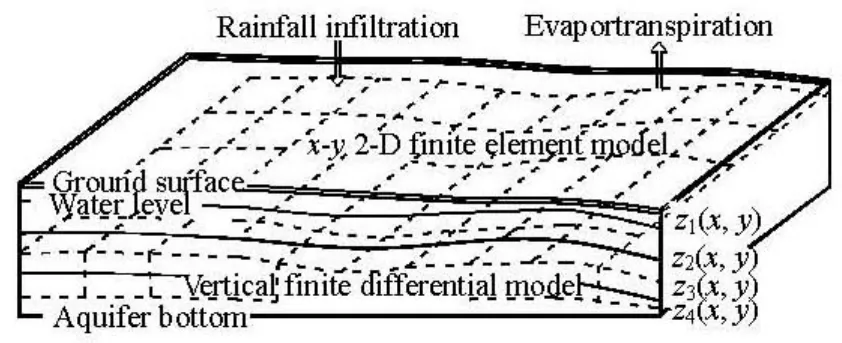
Fig.1 Schematic representation of structure of the simplified model

In each virtual layer Eq.(1) is integrated from top to bottom of aquifer along thez-axis and the thickness isM(x,y). According to Darcy’s law, we get the following 2-D water flow equation with the hypothesis of isotropy.

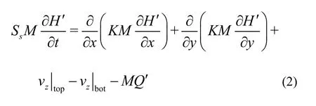
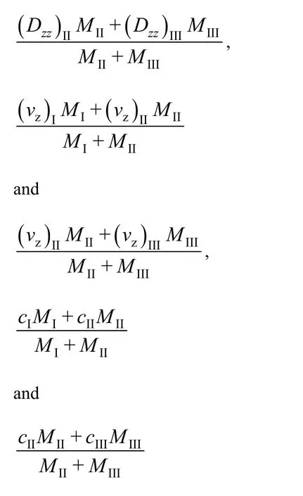
In Eq.(2), the following expressions are introduced:

In the layer which groundwater table lies, lower limits of the above integrals are notz=zi(x,y) but vertical coordinates of groundwater table.vz|topand vz| bot are the vertical Darcy velocities through the top and bottom plane of each aquifer layer separately.

2.2Finite element matrix equation of the simplified

3-D flow model

The research areaΩof each layer is spatially discretized andφnis the linear base function of noden(n=1,2,NP). The Galerkin finite element expression of Eq.(2) is,

Equation (3) is accumulated in all finite elementseof each layer as the following matrix equation:

δnmis the Kronecker tensor,Aeis the area of elemente,andare the average saturated hydraulic conductivity and aquifer thickness of each layer,am,an,bm,bnare terms related with spatial coordinates of elemente,σ1nis the flux of the Neumann type boundary node andLnis boundary segment of the corresponding node, andQe′is the average sink/source of elemente. The full implicit formulation of time discretization of Eq.(4) is,

wherek+1 andkare the current time and the former time, Δtkis the time step,

Fig.2 Illustration of finite element matrix in the simplified model

2.3Coupling numerical algorithm and solution strategy

Suppose that the research area is divided intoNlayers, the aquiferous footwall stratum lies in LayerN, the ground surface is located in Layer 1 and number of nodes in each layer isn. After Eq.(2) has been spatially discretized based on the Galerkin FEM, a series of 2-D finite element matrices for each layer, i.e.,LI(I=1,,N), are formed (see Fig.2), the dimensions of the matrix of each layer are the same. The whole finite element matrix of the area is madeup of the basic matrix of each layer and physical coupling process is 3-D water balance of study area.

Taking an example for three layers and assuming that the free surface lies within the upper layer, we obtain the whole matrixL(see Fig.2), in which unaffected terms in the original 2-D matrix are denoted asljand those which are modified are

iwritten asLi

j(i,j=1,,3n). There would be a vertical hydraulic relationship between each node of Layer 1 and 2 and between each node of Layer 2 and 3. Therefore, in the following we give values for each node of Layer 2 of the whole matrix. The two expressions are obtained as follows:

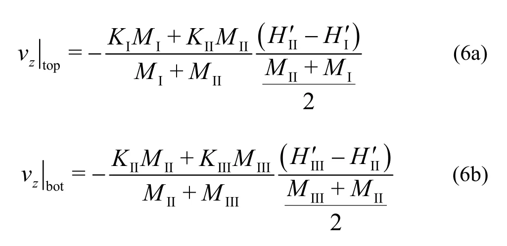
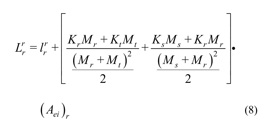
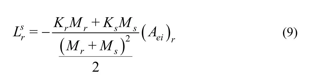
whereAeidenotes the controlling area of nodeiamong finite element grids.

Because the resulting matrix is nonlinear, an iterative process must be used to obtain the solutions of the global matrix equation at each new time step. The preconditioned conjugate gradient and ORTHOMIN method is used to solve the nonlinear system of matrix equations. After inversion, the coefficients matrix is re-evaluated using the first solution and the new equations are again solved. The iterative process continues until a satisfactory degree of convergence is achieved. The first estimate of the unknown hydraulic heads at each time step is obtained from the head values at the previous time level.

2.4Simulation of free groundwater surface

In the simplified model we keep the grids of each layer invariable during iteration. The physical essence of this method is that the thicknesses and velocity at the dry nodes in dry or partly dry layers are zero[15]. To ensure stabilization and avoid overflow, we set the thicknesses of those dry nodes as a small value (about 0.05 m) according to the supposed groundwater table at current timetk+1, and the computation of other nodes is not disturbed.

2.5Effects of complicated boundary and medium conditions

The setting of each layer in the supposed model should be concerned during solving complicated boundary conditions and heterogeneous medium. Virtual conductance parameters can be considered as a solving method of river, stream, drain and horizontal flow barrier flow boundary conditions. Interpolation with the depth of recharge and evapotranspiration can be added into sink/source term of the simplified model. For the complicated medium conditions, such as fault existing in large scale groundwater system, the structure definition of the aquiferous layer can take the virtual method. It means that the strata of both sides of the fault should virtually extend to the whole boundary to get vertical multi-layer structure and the hydrogeology parameters in the fault should be set based on its hydraulic relation. ignored if the node is in the layer where groundwater

3. Description of the simplified solute module

3.1x-y 2-D CDE of each layer

Based on Fick’s law and solute mass conservation, the 3-D solute transport equation is

wherexi(i=1,2,3) are the spatial coordinates,θis the volumetric soil water content,cis the solute concentration,Dijis the dispersion coefficient tensor,viis thei-th component of velocity flux, andCsis the concentration of the solute in the injected water.

The governing equation in the simplified model is an integration ofx-y2-D CDE of each layer (i.e.,i=1,2in Eq.(10)). In order to keep 3-D mass balance in the computational domain, the convection flux and vertical solute dispersion flux should be added tox-y2-D solute transport equations of each layer. Therefore, we get the following equation:

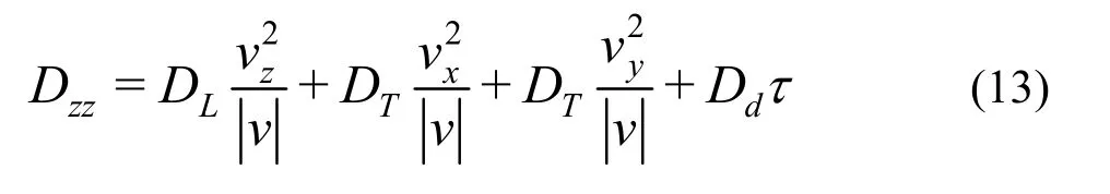
In the regional scale study of flow movement and solute transport, we assume that transport is mainly vertical and the corresponding error is neglected. The dispersion coefficients in thex-zandy-zplanes are not considered (Dxz=Dzx=Dyz=Dzy=0) in the proposed model. The four components of thex-y2-D dispersion tensor in the liquid phaseDij, are generally given by

3.2Finite element matrix equation of the simplified solute model

The 2-D Galerkin finite element expression of Eq.(11) in each layer is

Equation (13) is accumulated in all elementseof each layer as the following matrix equation:

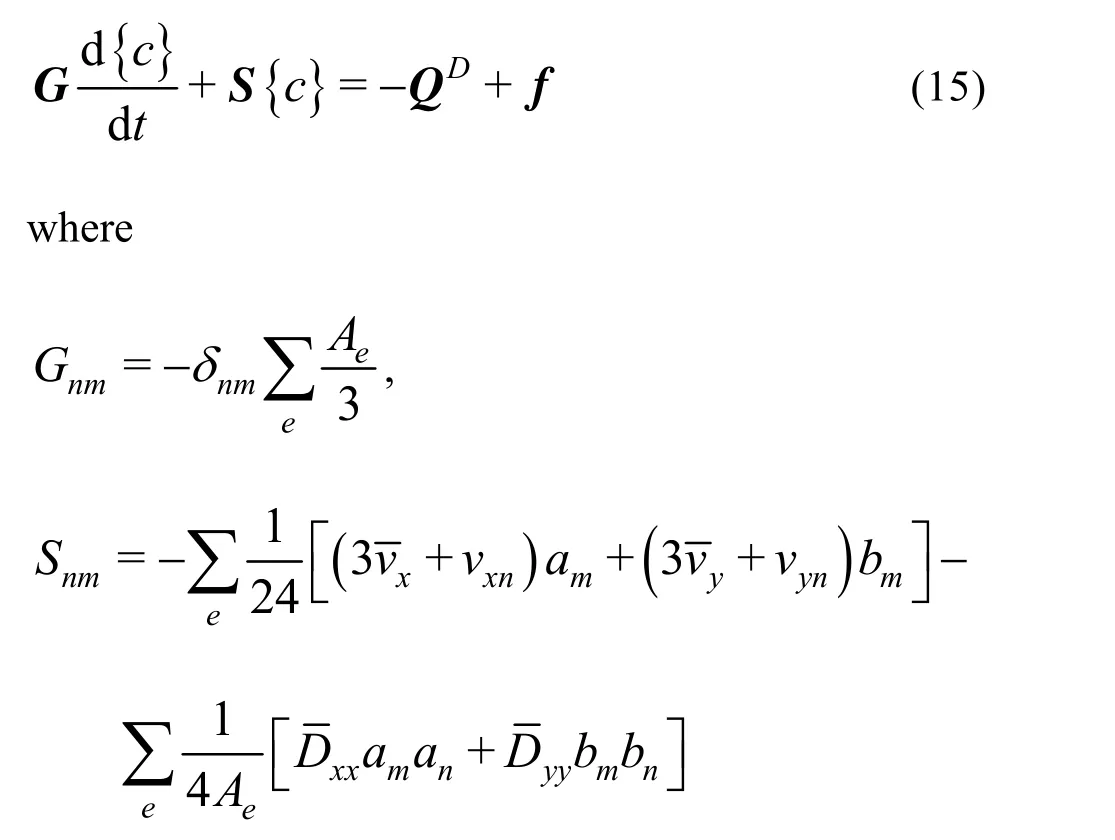
The dispersion flux QDfrom boundary integral is not briefly considered in time discretization of Eq.(15) and we can get,

3.3 Coupling numerical algorithm and solution strategy

The whole matrix structure for the simplified solute transport module is the same as that of the flow module (see Fig.2). In the matrix Eq.(16), the unaffected terms are denoted asand p andi those modified elements are written asandpi (i,j=1,,3n). In the following, we give the values for each node of Layer 2 of the whole matrix. The two expressions are given as

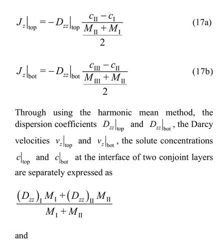
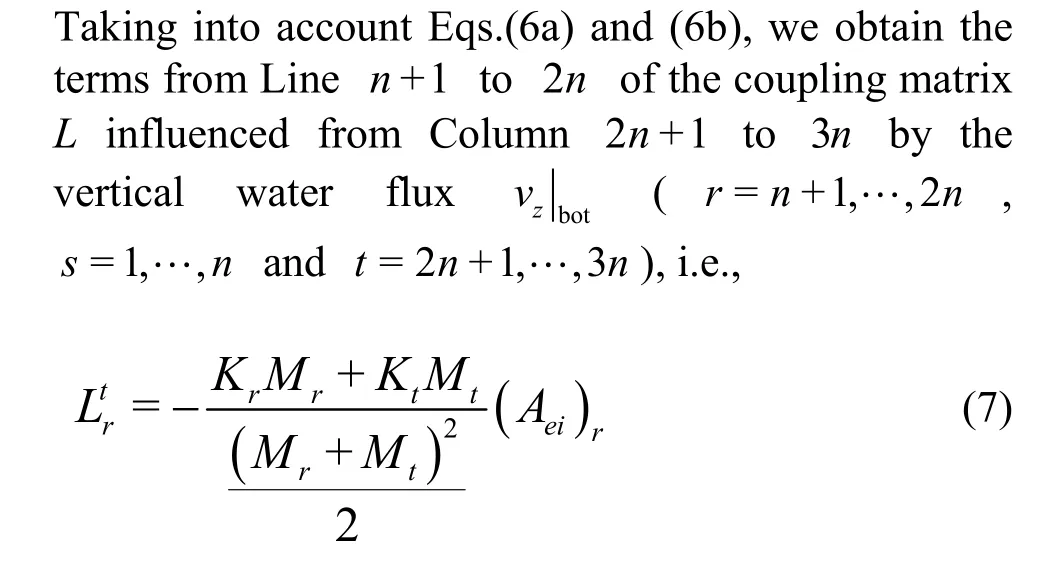
The components on Lines n+1 to 2n in the coupling matrix should be added the impact of vertical solute flux from Column 1 to n, from Column n+1to 2n and from Column 2n+1 to 3n in turn, i.e.,

And the right vector of Eq.(16) is modified as

The solution process at each time step proceeds as follows. After achieving the convergence of the simplified flow module, the solution of the simplified solute module is implemented. This is done by first determining the nodal values of the fluid flux from nodal values of the hydraulic head by applying Darcy’s Law. The values for the fluid flux is subsequently used as input to the transport Eq.(16) which was modified according to the above mass balance process leading to a system of linear algebraic equations. The resulting equations are also solved by the preconditioned conjugate gradient and ORTHOMIN method.

4. Model verification

4.1Test 1

The problem of a pumping well was set to demonstrate the accuracy and precision of the simplified model. The cuboid flow domain is presented with a height of 25 m (from the aquifer lower bed to the soil surface) and a length and a width of 200 m. Initial groundwater level isH0=23m. Pumping well was assigned at the center of the flow domain. During 200 d, the intensity of pumping is 60 m3/d and the screen length of the well-bore is from 13 m to 25 m under the ground surface. After steady state had reached, pumping ceased and water level began to rise. The boundary conditionH=23m for flow is specified around the area. The saturated hydraulic conductivity is 0.2975 m/d. The grid steps along thexandycoordinates are 1 m×20 m, 4 m×12.5 m, 4 m×5 m, 10 m×2 m, 4 m×5 m, 4 m×12.5 m, 1×20 m. The grid steps along thezcoordinate from the aquifer lower bed to the ground surface are 12 m, 6 m, 1.5 m, 3 m×1 m, and 2.5 m.

For easy comparison with the Visual Modflow[7], the same spatial interval is taken in the two models and the first vertical layer below the soil surface includes the initial phreatic surface. The time step in the simplified model is from 0.01 to 5 d according to the numerical iteration and the length of each stress period in the Visual Modflow is also 5 d. The convergence criterion of hydraulic head in the two models is 0.01 m. The solver for the flow simulation in the Visual Modflow is the WHS Solver which uses a Bi-Conjugate Gradient Stabilized acceleration routine.

During pumping, groundwater table gradually decreases from constant pressure head boundaries to the center of seepage area and the absolute error of groundwater level between the two models is small. After 200 d, water table remains steady and spans 5 layers (see Fig.3). This indicates that the simplified model can simulate the changes of water level which is lower than floor of each layer. And it is exact when dealing with water exchange between different layers.

Fig.3 Groundwater level at 100 m away from constant head boundary (The simplified model is signed as dashed line, Modflow is real line and boundary of each layer is dash-dotted line)

The changes of total head with time can be simulated by the two models by setting observation nodes (see Fig.4). Those nodes have different distances from the well and all lie in the first layer. The number of layers for groundwater level spans is related to the distance from the pumping well, which is following with the station of groundwater table of each node. Pumping steady state at the time of 200 d is taken as initial condition of backwater, which is close to steady state again at the time of 400 d. At last, the results of the simplified model are closer to the initial water table than those of Modflow.

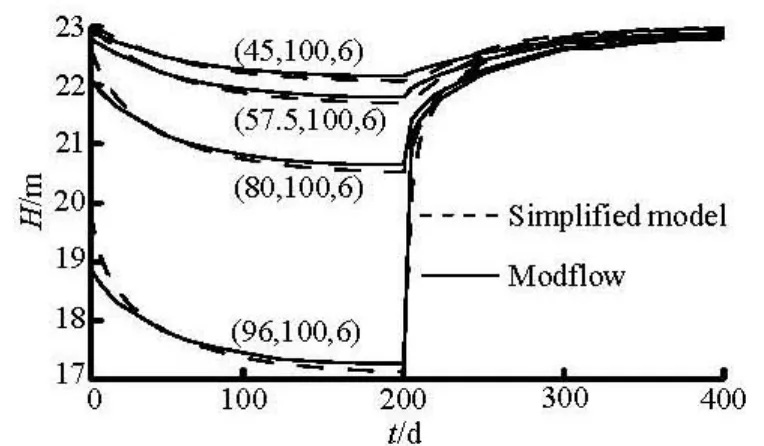
Fig.4 Pumping and backwater curves at different observing nodes

The cumulative pumping water, flux along the Dirichlet boundary, flux increment in the seepage area and absolute error are presented. They are labeled as Pump, Dirichlet, Volume and WBalT separately in Fig.5. The relative error (WBalR) is near zero which proves the simplified model keeps water balance well.

Table 1 Soil hydraulic and solute properties in Test 2

4.2Test 2

Fig.5 Water balance of pumping and backwater process with the simplified model

Fig.6 Illustration of the simulated area is shown, the upper part is x-y plane and the lower part is x-z plane (unit: m)

An equivalent finite differential grid is implemented for simulations with the Modflow and MT3DMS (included in the Visual Modflow). The time step in the simplified model is from 0.01 to 1 day according to the numerical iteration. The lengths of ten stress periods in the Visual Modflow are all 730 d and each includes 730 time steps. The convergence criterion of hydraulic head in the two models is 0.01 m. The solver for the flow simulation via the Visual Modflow is the WHS Solver and the Generalized Conjugate Gradient (GCG) Solver with the central finite difference method is used for achieving transport variants in MT3DMS.

As far as the water flow module is concerned, the station of groundwater surface is compared (see Fig.7). It is shown that the absolute error and the relative water balance error are reasonable. Solute concentration plume of plane sections and vertical profiles are illustrated (see Figs.8 and 9). The maximum relative error of concentration is 0.5%.

Compared with the Visual Modflow, the computation efficiency of the simplified model has a good presentation. The imaginary case is computed by a PC with the CPU of 2.8 GHz and the EMS memory of 512 MB. From Table 2, it can be seen that the simplified model uses more processor time than the Visual Modflow when solving flow problem. The longer run time in the simplified model is cost for modifying and updating the integrated matrix equation. However, the solute transport simulation of thesimplified model is more efficient than the Visual Modflow, and run time savings are considerable. This is because the time spent modifying the integrated equations is only a small fraction of the overall computational effort. Thus, transport model run time savings of 83% is achieved. The overall run time savings (accounting for both flow and transport model) are virtually the same as the run time savings for the transport model alone (71%).

Fig.7 Groundwater table of the whole seepage area after 7300 d

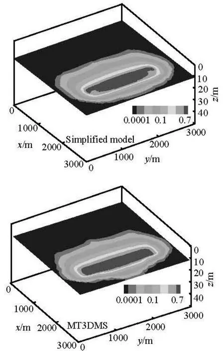
Fig.8 Concentration plume at the 4th layer (10.5 m below ground surface) after 7300 d

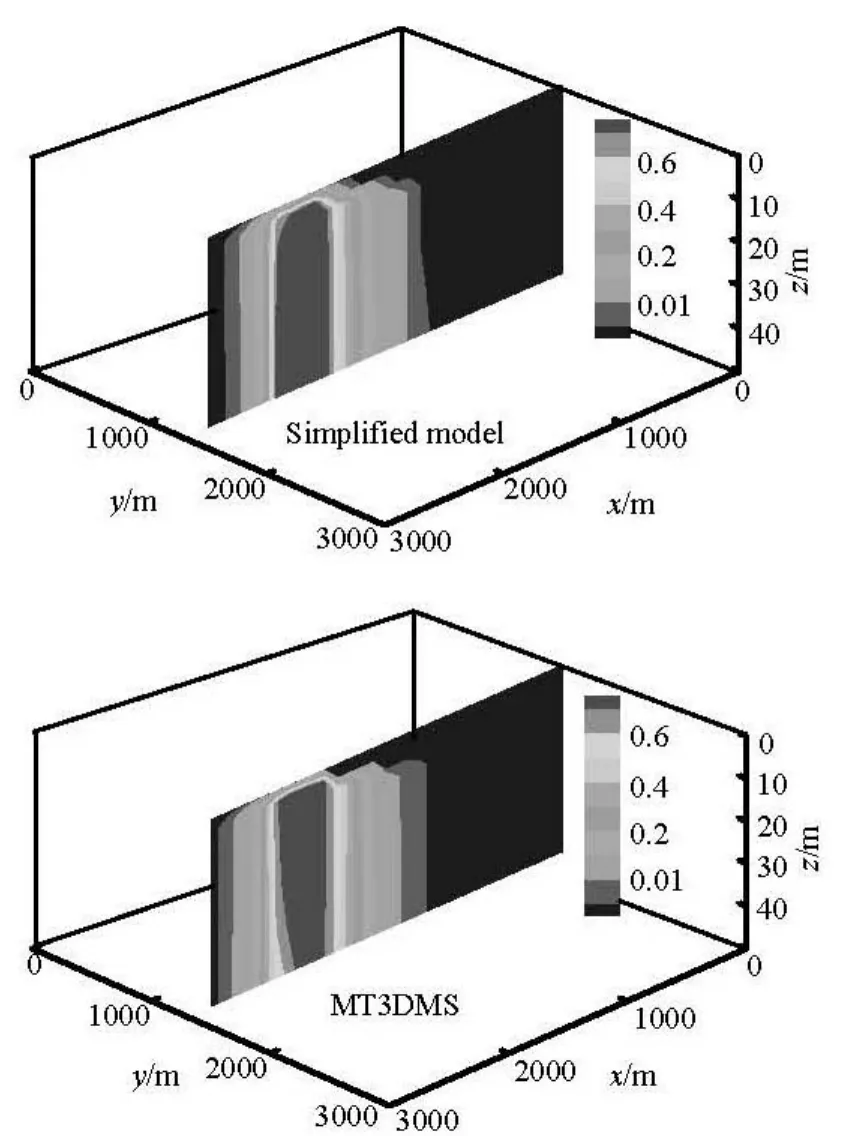
Fig.9 Solute concentration plume of vertical profiles after 7300 d (1500 m from the boundary)

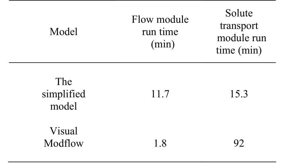
Table 2 Comparision of the simplified model and Visual Modflow run times

The MT3DMS supports an alternative form which allows the use of two transverse dispersivities, a horizontal transverse dispersivity (DTH) and a vertical one (DTV) as was proposed by Burnett and Frind[16]. Accordingly, there are nine components of the 3-D dispersion tensor in the MT3DMS. In the presented simplified model, the hypothesis that solute transport is mainly vertical between virtual layers willcause computation error. Therefore, the simplified model is not suitable when solute transport is highly 3-D.

5. Conclusions

Based on the integration of 2-D finite element method in thex-yplane and 1-D finite differential method along thezdirection, a simplified groundwater and solute transport numerical model at large scale has been developed. The model redistributes finite element matrices to improve computation efficiency. In the two studied cases, the simulated results comparison between the simplified model and Visual Modflow is presented. It stresses good results on dynamic station of groundwater table, transient head of observation points, and water balance and solute plume. The numerical algorithm of the simplified model is proved to be accurate and steady. When predicting solute plume, high computation efficiency is achieved with the simplified model.

Compared with the full 3-D model, the simplified model is easily to compile the source code, saves memory space, has an effective solution to discretized system of equations and depicts non-stationary 3-D situation of groundwater table and solute plume. Thus the simplified model is with great suitability of natural non-horizontal and heterogeneous aquifer condition.

[1] ALMASRIA M. N., KALUARACHCHI J. J. Modeling nitrate contamination of groundwater in agricultural watersheds[J].Journal of Hydrology,2007, 343(3-4): 211-229.

[2] LIU Xiao-bo, PENG Wen-qi and HE Guo-jian et al. A coupled model of hydrodynamics and water quality for Yuqiao Reservoir in Haihe River Basin[J].Journal of Hydrodynamics,2008, 20(5): 574-582.

[3] JULIAN H. E., BOGGS M. and ZHENG C. M. et al. Numerical simulation of a natural gradient tracer experiment for the natural attenuation study: Flow and physical transport[J].Ground Water,2001, 39(4): 534-545.

[4] TAN Ye-fei, ZHOU Zhi-fang. Simulation of solute transport in a parallel single fracture with LBM/MMP mixed method[J].Journal of Hydrodynamics,2008, 20(3): 365-372.

[5] PARK E., ZHAN H. B. Analytical solutions of contaminant transport from finite one-, two-, and three-dimensional sources in a finite-thickness aquifer[J].Journal of Contaminant Hydrology,2001, 53(1-2): 41-61.

[6] REFSGAARDA J. C., THORSENA M. and JENSENA J. B. et al. Large scale modeling of groundwater contamination from nitrate leaching[J].Journal of Hydrology,1999, 221(3-4): 117-140.

[7] MCDONALD M. G., HARBAUGH A. and MODFLOW W. Modular three-dimensional finite-difference ground-water flow model. 6. Appendix A-1-A-2[R]. U.S. Geological Survey, 1999.

[8] ZHANG Qian-fei, LAN Shou-qi and WANG Yan-ming et al. A new numerical method for groundwater flow and solute transport using velocity field[J].Journal of Hydrodynamics,2008, 20(3): 356-364.

[9] BERENDRECHT W. L., HEEMINK A. W. and Van GEER F. C. et al. A non-linear state space approach to model groundwater fluctuations[J].Advances in Water Resources,2006, 29(7): 959-973.

[10] KARAHAN H., TAMER A. M. Transient groundwater modeling using spreadsheets[J].Advances in Engineering Software,2005, 36(6): 374-384.

[11] TREFRY M. G., MUFFELS C. FEFLOW: A finiteelement ground water flow and transport modeling tool[J].Ground Water,2007, 45(5): 525-528.

[12] BANDILLA K. W., JANKOVI?A I. and RABIDEAU A. J. A new algorithm for analytic element modeling of large-scale groundwater flow[J].Advances in Water Resources,2007, 30(3): 446-454.

[13] HUANG J. Q., CHRIST J. A. and GOLTZ M. N. An assembly model for simulation of large-scale ground water flow and transport[J].Ground Water,2008, 46(6): 882-892.

[14] KUO Y. C., HUANG L. H. and TSAI T. L. A hybrid three-dimensional computational model of groundwater solute transport in heterogeneous media[J].Water Resources Research,2008, 44(3): 179-191.

[15] ZHAO M. D., LI Y. T. and QIU H. M. et al. Numerical simulation study on influence of exploiting Hankou Beach flood control[J].Journal of Wuhan University of Hydraulic and Electric Engineering,2000, 33(4): 10-13(in Chinese).

[16] BURNETT R. D., FRIND E. O. Simulation of contaminant transport in three dimensions. 2. Dimensionality effects[J].Water Resources Research,1987, 23(4): 695-705.

July 1, 2009, Revised October 10, 2009)

* Project supported by the National Science Fund for Distinguished Young Scholars (Grant No. 40701071).

Biography:LIN Lin (1981-), Female, Ph. D., Associate Professor

2010,22(3):319-328

10.1016/S1001-6058(09)60061-5