
Coupling of the Calculated Freezing and Thawing Front Parameterization in the Earth System Model CAS-ESM
2023-09-07 07:49:22RuichaoLIJinboXIEZhenghuiXIEBinghaoJIAJunqiangGAOPeihuaQINLonghuanWANGandSiCHEN
Advances in Atmospheric Sciences 2023年9期
Ruichao LI, Jinbo XIE, Zhenghui XIE*,2, Binghao JIA*, Junqiang GAO, Peihua QIN,Longhuan WANG, and Si CHEN
1State Key Laboratory of Numerical Modeling for Atmospheric Sciences and Geophysical Fluid Dynamics,Institute of Atmospheric Physics, Chinese Academy of Sciences, Beijing 100029, China
2College of Earth and Planetary Sciences, University of Chinese Academy of Sciences, Beijing 101408, China
3School of Mathematics and Statistics, Nanjing University of Information Science and Technology, Nanjing 210044, China
ABSTRACT The soil freezing and thawing process affects soil physical properties, such as heat conductivity, heat capacity, and hydraulic conductivity in frozen ground regions, and further affects the processes of soil energy, hydrology, and carbon and nitrogen cycles.In this study, the calculation of freezing and thawing front parameterization was implemented into the earth system model of the Chinese Academy of Sciences (CAS-ESM) and its land component, the Common Land Model(CoLM), to investigate the dynamic change of freezing and thawing fronts and their effects.Our results showed that the developed models could reproduce the soil freezing and thawing process and the dynamic change of freezing and thawing fronts.The regionally averaged value of active layer thickness in the permafrost regions was 1.92 m, and the regionally averaged trend value was 0.35 cm yr—1.The regionally averaged value of maximum freezing depth in the seasonally frozen ground regions was 2.15 m, and the regionally averaged trend value was —0.48 cm yr—1.The active layer thickness increased while the maximum freezing depth decreased year by year.These results contribute to a better understanding of the freezing and thawing cycle process.
Key words: frozen ground, freezing and thawing fronts, maximum freezing depth, active layer thickness, earth system model CAS-ESM
1.Introduction
Frozen ground is widely distributed in the northern hemisphere, accounting for about 50% of land area, where soil freezing and thawing processes play an important role in terrestrial ecosystems.It can affect snow cover (Rawlins et al.,2005; Iwata et al., 2010), the energy exchange between the land surface and atmosphere (Delisle, 2007; Yang et al.,2010; Guo et al., 2011a, 2017b), hydrological processes(Cherkauer et al., 1999; Guo et al., 2011b; Cuo et al., 2015;Zhao et al., 2018), the productivity of the vegetative growth season (Kim et al., 2012; Wang et al., 2015), the carbon cycle of terrestrial ecosystems (Koven et al., 2009; Schuur et al., 2008, 2015), and regional and global climate (Chen et al., 2014; Qin et al., 2014; Biskaborn et al., 2019).In soil freezing and thawing cycles, a boundary exists between frozen and unfrozen, namely the freezing and thawing front(Wang et al., 2014; Gao et al., 2019).With the change of soil freezing and thawing fronts, soil’s thermodynamic and hydraulic properties drastically change.If soil freezes, soil water is transformed into soil ice, which increases the thermal conductivity of soil and decreases its hydraulic conductivity,thus affecting the hydrothermal process of soil.The freezing fronts of soil affect snow infiltration during melting (Iwata et al., 2010).The change in the maximum freezing depth of seasonally frozen ground region affects engineering construction in the frozen region (Takata and Kimoto, 2000).The maximum thawing depth, also called the active layer thickness,greatly affects the energy process, hydrological process, carbon and nitrogen cycles, climate change, and engineering construction in the permafrost regions (Brown et al., 2000; Nelson et al., 2004; Chen et al., 2014; Guo et al., 2017, 2017a;Qin et al., 2017; Peng et al., 2018).Therefore, accurately obtaining the change information of soil freezing and thawing fronts is significant in studying the energy, hydrological, carbon and nitrogen cycle processes, as well as infrastructure construction practices in permafrost regions (Gao et al.,2019; Li et al., 2021).
Simulations of frozen ground have improved considerably.Gao et al.(2016, 2019) developed a two-direction Stefan’s algorithm to simulate the dynamic change of the soil freezing and thawing fronts in the land surface model CLM4.5 (Oleson et al., 2013).Xie et al.(2018, 2020) developed a land surface model of the Chinese Academy of Sciences (CAS-LSM) that considers soil freezing and thawing fronts dynamics based on the Community Land Model,which has been applied to frozen ground simulations (Xie et al., 2021; Wang et al., 2021).However, there is little quantitative description concerning the dynamic change of soil freezing and thawing fronts in the land surface model, CoLM(Dai et al., 1997, 2003), and earth system model, CAS-ESM(Zhang et al., 2020).Explicit freezing and thawing fronts in land surface and earth system models would enable realistic simulations of soil temperature, soil moisture, and runoff/infiltration, thereby elucidating upon energy, water, and greenhouse gas exchange processes in high latitudes.
In this study, we implemented the calculated freezing and thawing front parameterization into the latest version of CoLM and CAS-ESM.We used this model to analyze the spatial and temporal distribution of freezing and thawing fronts and discuss the resultant effects on soil temperature.The remainder of this paper is organized as follows.Section 2 describes the model development, and section 3 outlines the experimental design.Section 4 evaluates the results, and section 5 provides a conclusion and a related discussion.
2.Model Development
2.1.The multi-layer soil Stefan algorithm
In this study, the multi-layer soil Stefan algorithm is used to calculate the depth of freezing and thawing fronts.This method was developed by Woo et al.(Woo et al.,2004; Xie and Gough, 2013).
The common form of the Stefan equation is given by:
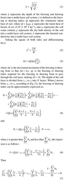
whereirepresents the number of soil layers andzirepresents the node depth of the soil layer.Equation (9) is the expression that can be applied to calculate the depth of the freezing and thawing fronts in multi-layered soil.When the depth of soil freezing or thawing, ξ, does not exceed the first layer of soil,the traditional Stefan formula is applied.When the depth of soil freezing or thawing, ξ, exceeds the first layer of soil,the multi-layer soil Stefan algorithm is applied.The freezing or thawing index is needed to judge which layer the freezing or thawing depth, ξ, is located inI.
2.2.CAS-ESM and CoLM
CAS-ESM is comprised of an atmospheric circulation model, an ocean model, a sea ice model, and a land surface model (Zhang et al., 2020).Its component models are mainly composed of the atmospheric general circulation model IAP AGCM of the Institute of Atmospheric Physics,Chinese Academy of Sciences, the climate system ocean model LICOM of the Institute of Atmospheric Physics, Chinese Academy of Sciences, the land surface process model CoLM of Beijing Normal University, the sea ice model CICE of Los Alamos Laboratory, the climate research and prediction model WRF, etc.Different component models are connected through the coupler of the Community Earth System Model.At the same time, it has also participated in the international coupling model comparison program CMIP6 (Zhang et al., 2020) as China’s earth system model and has performed well in the international coupling model comparison program.
The land surface model, CoLM, is developed from the initial version of the general land surface model CLM.CoLM is mainly developed and maintained by Chinese researchers, and its performance is relatively reliable worldwide, considered one of the land surface models with perfect functions (Dai et al., 2003, 2004, 2014).CoLM has been widely used in simulating land surface ecological processes,carbon cycle processes, hydrological processes, and energy processes.Recently, it has also participated in the Coupled Model Intercomparison Program (CMIP6) as the land component of the earth system model BNU-ESM of Beijing Normal University, the general comprehensive evaluation earth system model of Tsinghua University, and the earth system model CAS-ESM of the Chinese Academy of Sciences (Ji et al., 2014; Zhang et al., 2020).Regarding the soil freezing and thawing process, the freezing and thawing parameterization scheme of CoLM has been greatly improved (Xiao et al., 2013).However, there is still a lack of description of the important variable of soil freezing and thawing fronts,which is very important for reasonably expressing soil freezing and thawing processes in the model.
2.3.Implementation of the multi-layer soil Stefan algorithm in CAS-ESM
In this study, the multi-layer soil Stefan algorithm was added to the soil temperature module of the land surface model, CoLM, in the coupled CAS-ESM.Permafrost refers to the types of rocks and soil that contain ice; the upper layer thaws in summer, freezes in winter, and the lower layer remains frozen all year round.In permafrost, the frozen ground begins to thaw in spring when soil-thawing fronts appear.The frozen ground continues to thaw and reaches its maximum thawing depth in summer.The frozen ground begins to freeze again in autumn when the soil freezing fronts begin to appear.In winter, the frozen ground completely freezes, and no freezing or thawing fronts exist.The seasonally frozen ground is rock and soil that freezes in the winter and thaws completely in the summer.In the seasonally frozen ground region, the frozen ground begins to freeze in autumn when soil freezing fronts begin to appear.In winter,the frozen ground continues to freeze and reaches its maximum freezing depth.In spring, the frozen ground begins to thaw as soil-thawing fronts appear.The frozen ground thaws completely so that the summer has no freezing or thawing fronts.So the change of freezing and thawing fronts differs for permafrost and seasonally frozen ground.Therefore, we must distinguish between permafrost and seasonally frozen ground before simulating freezing and thawing fronts.
A model grid cell is identified as containing permafrost if at least one soil layer within the upper 10 layers remains frozen throughout the year (10 layers equates to 3.8-m depth).A model grid cell is considered seasonally frozen ground when we identify at least one monthly frozen soil layer during the climatological ensemble mean annual cycle(Lawrence et al., 2012).It should be noted that the definition of permafrost is more consistent with near-surface permafrost in this paper because the simulated maximum depth of CoLM is 3.8 m.In permafrost, we simulated two freezing fronts and one thawing front.One of the freezing fronts was the virtual front set, and the depth of this freezing front was 3.8 m, which does not actually exist.Rather, the intent in this particular identification is to distinguish between permafrost and seasonally frozen ground, noting that in seasonally frozen ground regions, one freezing front and one thawing front are simulated
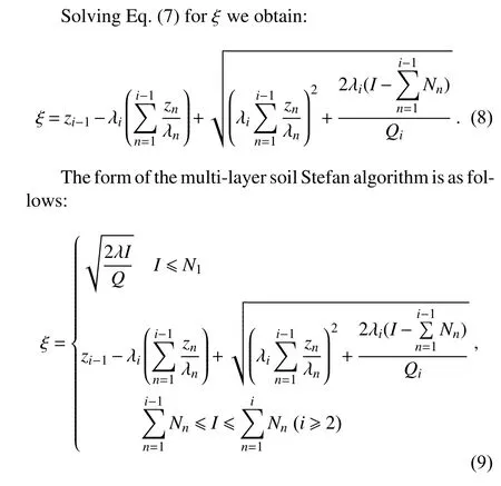
When the soil begins to freeze or thaw, we calculate soil freezing or thawing fronts by the multi-layer soil Stefan algorithm.Then, we updated the soil layer stratification by adding the depth information of soil freezing or thawing fronts, as is shown in Figs.1b and c.Noting that there are 15 soil layers in CoLM, we updated the soil layer stratification by adding the depth information of soil freezing or thawing fronts, as shown in Fig.1c.After adding the depth information of soil freezing or thawing fronts, the soil-layer stratification of CoLM added one new layer, so that CoLM now contains 16 layers (Fig.1c).The originalilayer andi+1 layer became the newjlayer,j+1 layer, andj+2 layer by adding the depth information of soil freezing or thawing fronts.The thickness and depth of the added soil layer were calculated by the original CoLM layering method.The heat capacity and heat conductivity of the added soil layer were calculated in the same way as in the original CoLM.When the soil layer is thicker, the soil layer becomes thinner after adding the depth information of soil freezing or thawing fronts.
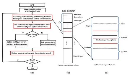
Fig.1.Schematic diagram of calculating soil freezing and thawing fronts in the land surface model, CoLM, of CAS-ESM.
We first calculated the soil temperature of the 16 layers by the heat equation.Then the soil temperature of the 16 layers was returned to the temperature of the original 15 layers,using the constant energy contained within.This is because the energy in the newjlayer,j+1 layer, andj+2 layer is equal to that of the originalilayer andi+1 layer at the same time.In this way, we are able to retain the soil temperature of the original 15 layers.We updated the soil layer stratification by adding the depth information of soil freezing or thawing fronts, primarily because the soil stratification in land surface model CoLM is thinner on top and thicker on the bottom.The land surface model CoLM uses the isothermal method to simulate the phase transition process; that is, the hydrothermal characteristics are assumed to be consistent within the same soil layer, and the phase transition only occurs at the central point of the soil layer.When this assumption is applied to thicker soil layers, the simulated soil freezing and thawing process can be either delayed or advanced.So when the soil layer is thicker and appears to be undergoing the freeze-thaw process, we added the location information of freezing or thawing fronts to the thicker soil layer so that the stratification of the thicker soil layer can be improved and become thinner.The soil temperature of the thicker soil layer can be improved using this method.The coupling process is illustrated in Fig.1.
3.Experimental Design
In this study, the land surface model CoLM was used for offline numerical experiments, which allowed us to simulate the soil freezing and thawing fronts and determine the influence of the freeze or thaw module on the simulated soil temperatures.The land surface model, CoLM, is driven by atmospheric forcing data from CLMQIAN(Community Land Model QIAN forcing data).The atmospheric forcing data include temperature, wind speed, humidity, solar radiation, and precipitation for 1948—2004.First, a 100-year spinup is conducted by duplicating the forcing data of 1948, and the simulation results obtained were taken as the initial value of mode operation.The simulation period was 1948—2004, with a resolution of 1.4° × 1.4°, and an analysis period between 1990—2000.It mainly analyzes the monthly and interannual changes of soil freezing or thawing fronts,so the soil freezing or thawing fronts are simulated and comprise output along with monthly scaled variables.
In all, three groups of experiments were conducted: (1)the soil layer was updated using the additional freezing front’s location information, (2) the soil layer was updated using the additional thawing front’s location information,and (3) the original soil layer was not updated with any freeze or thaw fronts information.The other settings (such as the simulation area, step size, and initial field) for both experiments were the same.The formal simulation output results had a monthly resolution.Meanwhile, the earth system model CAS-ESM was used to simulate the active layer thickness across the globe.The resolution for the land and atmosphere in these simulations was 1.4° in both latitude and longitude.
4.Evaluation and Application
4.1.The temporal and spatial distribution of soil freezing and thawing fronts
The section shows the temporal and spatial distribution of soil freezing and thawing fronts.
Figure 2 shows the simulated multi-year average spatial distribution of monthly thawing fronts depth from 1990 to 2000.As seen in the figure, there were partial thawing fronts in January, February, and March because the freezing fronts had not reached the maximum thawing fronts depth at this time.Starting in March, the temperature rises as frozen ground begins to thaw; consequently, thawing fronts appear.At this time, the thawing fronts mainly appear in the seasonally frozen ground region.As the temperature continues to rise, the depth of the thawing fronts increases, generally reaching their maximum thawing depth in September and October.At this time, the thawing fronts mainly exist in the permafrost region and gradually become more shallow from low to high latitudes.During the same time, the thawing fronts in the seasonally frozen ground region completely disappear, mainly because they have reached the maximum freezing front depth of the previous period when the frozen ground completely thaws and the fronts disappear.The thawing fronts of the permafrost region begin to disappear in November and December.As the temperature continues to decrease, the freezing fronts reach their maximum thawing front depth, causing the thawed soil to freeze completely and the thawing fronts to disappear.At this time, there were partial thawing fronts because the freezing fronts had not yet reached the maximum thawing front depth.
Figure 3 shows the simulated multi-year averaged spatial distribution of monthly freezing fronts depth in soils from 1990—2000 for the months of (a) September, (b) October, (c)November, (d) December, (e) January, and (f) February.Soil-freezing fronts mainly appear in late autumn and winter.At this time, the freezing fronts distribute themselves in the permafrost region, which is the actual freezing front of the two freezing fronts, while the freezing fronts in the seasonally frozen ground region are shown in Figs.3g—l.Figures 3a—f show that as the temperature begins to decrease in October, the frozen ground begins to freeze, and the freezing fronts begin to appear.At this time, the freezing fronts are primarily distributed in high latitudes and the Qinghai Tibet Plateau.As the temperature continues to decrease,the depths of the freezing fronts deepen.At this time, the freezing fronts at high latitudes begin to gradually disappear,mainly because the depths of the freezing fronts have reached the depth of the thawing fronts from the previous period.When the frozen ground is completely frozen, the freezing fronts disappear.There were still freezing fronts in January, indicating that the thawing fronts from the previous period in these areas must have been deep so that the depth of the freezing fronts have not reached the depth of the thawing fronts of the previous period.When the depth of the freezing fronts completely reaches the depth of the thawing fronts of the previous period, the freezing fronts disappear,and the frozen ground is considered completely frozen.During (g) November, (h) December, (i) January, (j) February,(k) March, and (l) April, the freezing fronts of permafrost were the previously set virtual fronts (most of the red areas),and the depth of the freezing fronts is 3.8 m, which do not actually exist.Therefore, only the freezing fronts in the seasonally frozen ground region are analyzed.As can be seen from Figs.3g—l, the temperature begins to decrease in November, the ground begins to freeze, and the freezing fronts begin to appear.With continually decreasing temperatures,the depths of the freezing fronts deepen, and the seasonally frozen ground region essentially reaches its maximum freezing depth in February.The spatial pattern of these freezing fronts are characterized by a gradual deepening from low to high latitudes.
To show the differences between freezing and thawing fronts more intuitively in permafrost and seasonally frozen ground, we also present the regional mean monthly profiles(line plot) of the depths of the freezing and thawing fronts of the permafrost and seasonally frozen ground.
We chose two grid points.One is located at 48.9°N,52.3°E, and is a representative point of seasonally frozen ground.The other one is located at 65.9°N, 137.8°E, and is a representative point of permafrost.Figure 4a shows simulated soil freezing and thawing fronts of seasonally frozen ground.The red line represents the change in the depth of soil freezing fronts, and the blue line is the change in the depth of soil thawing fronts.In the region of seasonally frozen ground, the frozen ground begins to freeze in November.The frozen ground continues to freeze and reaches its maximum freezing depth in February.The frozen ground begins to thaw in March.The frozen ground thaws completely, and there are no freezing or thawing fronts in June.Figure 4b shows the simulated soil freezing and thawing fronts of permafrost.The red line is the change in the depth of soil freezing fronts, and the blue line is the change in the depth of soil thawing fronts.The black line is the virtual soil freezing front.In permafrost, the frozen ground begins to thaw in June.The frozen ground continues to thaw and reaches its maximum thawing depth in September.The frozen ground begins to freeze in October on its way to freezing completely; consequently, there are no freezing or thawing fronts in January.The black line in Fig.4 represents the change in depth of the virtual soil freezing front, noting that the depth of this freezing front is 3.8 m, which does not actually exist; rather, this is the depth threshold that distinguishes between permafrost and seasonally frozen ground.
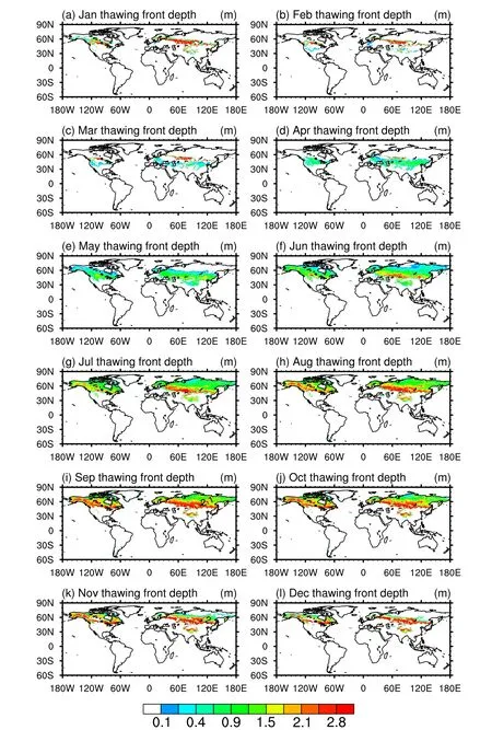
Fig.2.Simulated multi-year mean spatial distribution of the monthly thawing fronts depth (m) from 1990—2000.
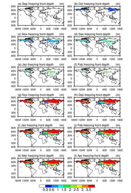
Fig.3.Simulated multi-year mean spatial distribution of monthly freezing fronts depth (m) from 1990—2000, (a)—(f): the distribution of freezing fronts in the permafrost region, (g)—(l): the distribution of freezing fronts in the seasonally frozen ground region.
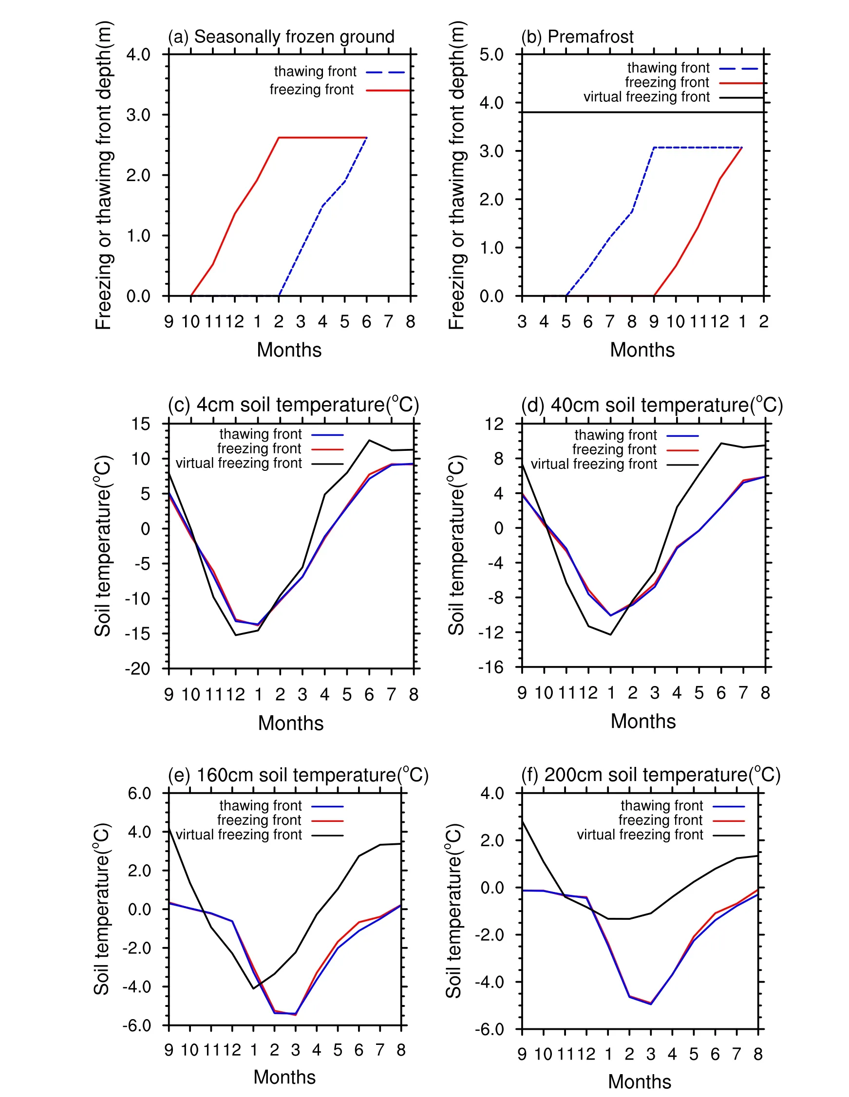
Fig.4.Simulated soil freezing and thawing fronts in (a) seasonally frozen ground and (b)permafrost.The red line is the change in depth of soil freezing fronts, the blue line is the change in depth of soil thawing fronts, and the black line is the virtual soil freezing front.The lower panels show the observed and simulated soil temperatures at (c) 4 cm, (d) 40 cm, (e)160 cm, and (f) 200 cm.The red line is the simulated soil temperature by the updated model,the blue line is the simulated soil temperature by the original model, and the black line is the observed soil temperature.
The soil thawing fronts mainly appear in late spring,summer, and early autumn, and the soil freezing fronts mainly appear in late autumn and winter (Fig.2; Fig.3;Figs.4a, b).The soil thawing fronts essentially reach their maximum depth in September and October.At this time, the thawing fronts mainly exist in the permafrost region.At the same time, the maximum thawing depth is called the active layer thickness, which refers to the soil layer thawed in summer and frozen in winter in a permafrost region.It is a very important index for permafrost regions.The soil-freezing fronts basically reach their maximum depth in February,when there is mainly seasonally frozen ground in the region at this time.The maximum freezing depth in the seasonally frozen ground regions refers to the maximum freezing depth in winter.In the permafrost regions, we mainly study the change of active layer thickness.We mainly study the change of maximum freezing depth in seasonally frozen ground regions.The following discussions mainly analyze the changes in active layer thickness in permafrost regions and the maximum freezing depth in seasonally frozen ground regions.
The change in active layer thickness in permafrost regions affects the processes of energy, hydrology, and carbon and nitrogen cycles.In recent years, due to global warming,permafrost degradation has become serious, and the active layer thickness is increasing.Therefore, analyzing the change in active layer thickness in permafrost regions is significant in studying permafrost degradation.In this study,the active layer thickness is the annual maximum depth of simulated soil thawing fronts.
Figure 5 shows the simulated spatial distribution and change trend of active layer thickness, ground temperature,and 2-m air temperature in the near-surface permafrost region from 1990 to 2000.As seen from Fig.5a, except for the Qinghai Tibet Plateau, the simulated active layer thickness decreases with increasing latitude, and the active layer thickness is the largest in the area where the permafrost region and seasonally frozen ground region intersect.The regionally averaged value of active layer thickness in the permafrost regions was 1.92 m, and the active layer thickness in the Qinghai Tibet Plateau is relatively thick as a whole.As evident from Fig.5b, the trend of active layer thickness shows an increasing trend year after year, and the regionally averaged trend value was 0.35 cm yr—1.
Because the multi-layer soil Stefan method uses ground temperature to calculate the freezing and thawing depth to simulate the active layer thickness, the multi-year averaged spatial distribution of ground temperature in permafrost regions from 1990 to 2000 and the trend of ground temperature from 1990 to 2000 are also given.Notably, the active layer thickness in permafrost regions is closely related to the ground temperature in summer, evidenced by the consistency between the spatial distribution and change trend of ground temperature and the spatial distribution and trend of active layer thickness (Figs.5c, d).In areas with warmer ground temperatures, the active layers were thicker, while in those areas with colder ground temperatures, the active layers were shallower.The regionally averaged value of ground temperature was 12.95°C.The trend of ground temperature was positive, showing a regionally averaged trend value of 0.038°C yr—1.
As the ground temperature increases, the active layer thicknesses also increase.The increasing trend of ground temperature is consistent with the increasing trend of active layer thickness.The ground temperature is closely related to the 2-m air temperature, so the spatial distribution and trend of 2-m air temperature in permafrost regions from 1990 to 2000 are also given (Figs.5e, f).The spatial distribution and trend of the 2-m air temperature and those of ground temperatures were consistent in their spatial distributions.The regionally averaged value of the 2-m temperature is 11.68 °C, and the regionally averaged trend value is 0.032 °C yr—1.As the 2-m air temperature increased year by year, the ground temperature increased simultaneously, which led to increases in the active layer thickness.
In the seasonally frozen ground region, we were mainly concerned about the change in maximum freezing depth.Figure 6 shows the simulated multi-year average spatial distribution of maximum freezing depth, ground temperature,and 2-m air temperature in the seasonally frozen ground region from 1990 to 2000 and their associated trends.As seen from Fig.6a, the simulated maximum freezing depth increased along with increasing latitude.The maximum freezing depth occurred at the junction of the permafrost region and the region of seasonally frozen ground.The regionally averaged value of the maximum freezing depth is 2.15 m,and the trend of the maximum freezing depth decreased year after year, with a regionally averaged trend value of—0.48 cm yr—1(Fig.6b).
Similar to the analysis of the permafrost region, we also provide the multi-year averaged spatial distribution and trend of ground temperature and 2-m air temperature in the seasonally frozen ground regions from 1990 to 2000.It should be pointed out that the maximum freezing depth in seasonally frozen ground regions is closely related to the ground temperature in winter.Therefore, the ground temperature and 2-m air temperature in winter are given here.The spatial distribution of ground temperature was consistent with the spatial distribution of maximum freezing depth (Figs.6c,d).In areas with high ground temperature, the maximum freezing depth was shallow, and in areas with low ground temperature, the maximum freezing depth was deep.The regionally averaged ground temperature was —9.36°C.The trend of ground temperature was positive, increasing year by year,yielding a regionally averaged trend value of 0.022°C yr—1.The increasing trend of ground temperature was consistent with a decreasing trend of maximum freezing depth.Since the ground temperature is closely related to the 2-m air temperature, we also present the spatial distribution and variation trend of the 2-m temperature in the seasonally frozen ground region from 1990 to 2000.The spatial distribution and change trend of the 2-m air temperature and the spatial distribution and change trend of ground temperature were consistent in their spatial distribution.The regionally averaged value of 2-m temperature was —9.58°C, and the regionally averaged trend value was 0.020°C yr—1.As the 2-m temperature increased year by year, the ground temperature increased, and there was a commensurate decrease in the maximum freezing depth.
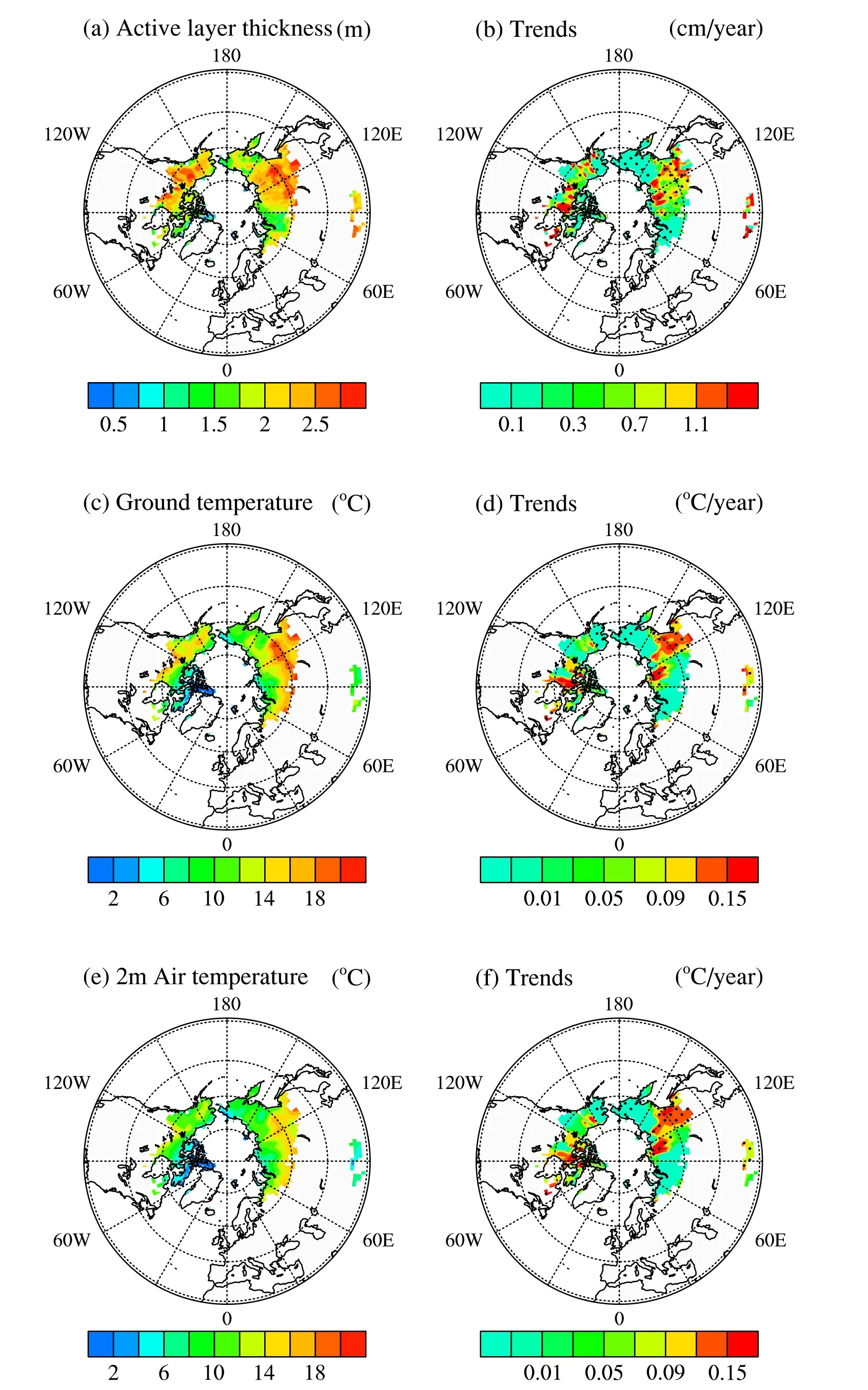
Fig.5.Spatial distribution of simulated (a) active layer thickness and (b) its trend, (c) ground temperature and (d) its trend, (e) 2-m air temperature and (f) its trend, from 1990 to 2000 in the permafrost region.
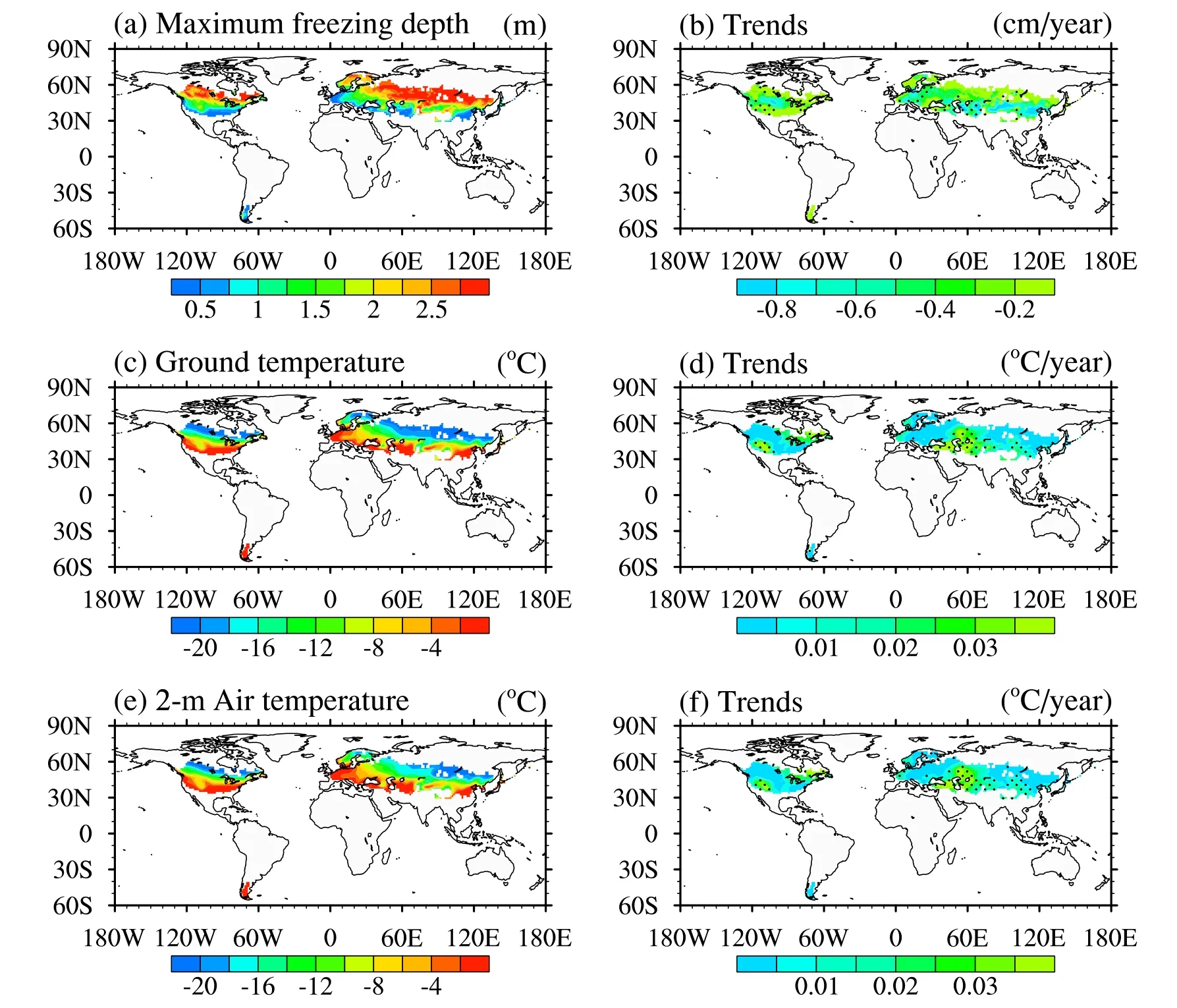
Fig.6.Spatial distribution of the simulated (a) maximum freezing depth and (b) its trend, (c) ground temperature and (d) its trend, (e) the 2-m air temperature and (f) its trend, from 1990 to 2000 in the seasonally frozen ground region.
4.2.The effect of soil freezing and thawing fronts on soil thermal processes
At first, we validated the simulated soil temperature with observed data.The observed data comes from station D66 in the northern part of the Qinghai-Tibet Plateau.It is located in the permafrost region.The soil temperatures were taken from 4 cm, 40 cm, 160 cm, and 200 cm depths from September 1997 to August 1998.These observational data are reliable and have been used to validate soil temperatures in other studies (Wang et al., 2014).The observed and simulated soil temperature at 4 cm, 40 cm, 160 cm, and 200 cm are shown in Figs 4c—f, respectively.The red line shows the simulated soil temperature by the updated model, the blue line shows the simulated soil temperature by the original model, and the black line shows the observed soil temperature.It can be seen that the correlation coefficients between the observed soil temperature and those simulated by the original model were 0.97, 0.93, 0.69, and 0.67 at 4 cm, 40 cm,160 cm, and 200 cm, respectively.The correlation coefficients between the observed soil temperature and those simulated by the updated model were 0.97, 0.93, 0.71, and 0.68 at 4 cm, 40 cm, 160 cm, and 200 cm, respectively.The root mean square difference between the observations and those simulated by the original model were 3.20°C, 4.06°C,2.82°C, and 2.34°C at 4 cm, 40 cm, 160 cm, and 200 cm,respectively.The root mean square differences between the observations and those simulated by the updated model were 3.23°C, 4.01°C, 2.69°C and 2.27°C at 4 cm, 40 cm,160 cm, and 200 cm.It can be seen that the simulated improvements in the deep soil are larger than that of shallow soil from the correlation coefficients and root mean square differences.The results are mainly attributed to the shallow soil layer being thin compared to the thicker deep soil layer.When the thawing fronts appear, we add the location information of the soil thawing fronts to the thicker soil layer, so the stratification of the thicker soil layer can be improved,thereby improving the simulations of the deep soil.
Additionally, we show the global-scale effect on the simulated soil temperature simulation.Three groups of global simulation tests were conducted and consisted of comparative control tests with and without considering the dynamic change of soil freezing and thawing fronts.First, we updated the soil layer using the location information of the additional freezing fronts.Second, we updated the soil layer using the location information of the additional thawing front.Third, the original soil layer was not updated with any freeze or thaw fronts information.The analysis year was 2000.
Figures 3g—l show that the freezing front of soil mainly occurs in winter.The global distribution of freezing depth is mainly shown for November, December, January, and February.As the temperature decreases in November, the ground begins to freeze, and a freezing front appears.At this time,the freezing fronts are mainly distributed in the seasonally frozen ground region.There is also a freezing front in the permafrost region, but it is a virtual front, or rather, only briefly exists; therefore, we only considered the freezing front in the seasonally frozen ground region.As the temperature continued to decrease, the depth of the freezing front began to deepen, and the maximum freezing depth was essentially reached in February.When the soil-freezing front appeared, we added it to the original soil stratification according to the location information of the soil-freezing fronts, restratified the soil layer, and changed the static stratification into dynamic stratification.
Figure 7 shows the soil temperature difference between different soil layers with and without a soil freezing front simulation in January.It is evident that adding the position information of soil freezing fronts to the original soil layer affects the soil temperature of different soil layers.In January, the soil freezing depth basically reached the eighth layer of soil depth.From the differences in soil temperature in different soil layers, it can be seen that it has a greater effect on the temperature simulation of deep soil and less of an effect on the temperature simulation of shallow soil.This was mainly because the shallow soil layer is thinner, and the deep soil layer is thicker.After adding the location information of the soil freezing front to the thicker soil layer, the stratification of the thicker soil layer can be improved, so the simulation was positively affected.
The change of soil temperature in different layers had a certain effect on ground temperature, latent heat flux, sensible heat flux, and soil humidity.Figures 9a—d show the difference in ground temperature, latent heat flux, sensible heat flux,and volumetric soil water in 2000.Such effects were consistent with the spatial distribution of soil freezing depth in Figs.3g—l.Although certain effects were observed on an annual timescale, they generally had little effect.
Figure 8 shows the soil temperature difference between the simulation with and without a soil-thawing front in July.It can be seen that adding the location information of soilthawing fronts to the original soil layer affected the soil temperature of different soil layers.In July, the soil thawing depth reached the eighth layer of soil depth.From the soil temperature difference of different soil layers, it can be seen that it had a greater effect on the soil temperature simulation of deep soil and less of an effect on the soil temperature simulation of shallow soil.This was mainly because the shallow soil layer is thinner, and the deep soil layer is thicker.After adding the location information of the soil thawing front to the thicker soil layer, the stratification of the thicker soil layer can be improved, so the simulation was positively affected.
Figures 9e—h show the differences in ground temperature, latent heat flux, sensible heat flux, and volumetric soil water for the year 2000.The effects of ground temperature,latent heat flux, sensible heat flux, and volumetric soil water were consistent with the spatial distribution of thawing depth in Fig.2.The annual average indicates that it had a certain effect on ground temperature, latent heat flux, sensible heat flux, and volumetric soil water, but overall, the effects were minimal.
This section mainly discusses the implications of either considering or neglecting the change of soil freezing and thawing fronts as they would influence simulated soil temperatures.The monthly spatial distribution of soil freezing and thawing fronts on a global scale and the soil temperature difference simulated with and without considering the change of soil freezing and thawing fronts were given.The simulated soil temperature difference indicates that it greatly affected the deep soil temperature.The reason is that we have improved the deep thicker soil layer and made it thinner by increasing the soil freezing or thawing fronts.In doing so,we improved the ability to simulate the deep soil temperature.From the annual average, it had a certain effect on surface temperature, latent heat flux, sensible heat flux, and volumetric soil water, but the effect was not significant.Further research is required to combine more observational data to discuss and consider the effect of changing soil freezing and thawing fronts on soil thermal processes to improve the simulation capability of hydrothermal processes within the land surface model.
4.3.The spatial distribution of active layer thickness from CAS-ESM
The earth system model CAS-ESM was used to simulate the active layer thickness across the globe.We analyzed the simulated spatial distribution of active layer thickness from 1990 to 2000.
As seen in Fig.10, except for the Qinghai Tibet Plateau,the simulated active layer thickness decreases with increasing latitude, and the active layer thickness is largest in the area where the permafrost region and seasonally frozen ground region intersect.
5.Discussion and conclusion
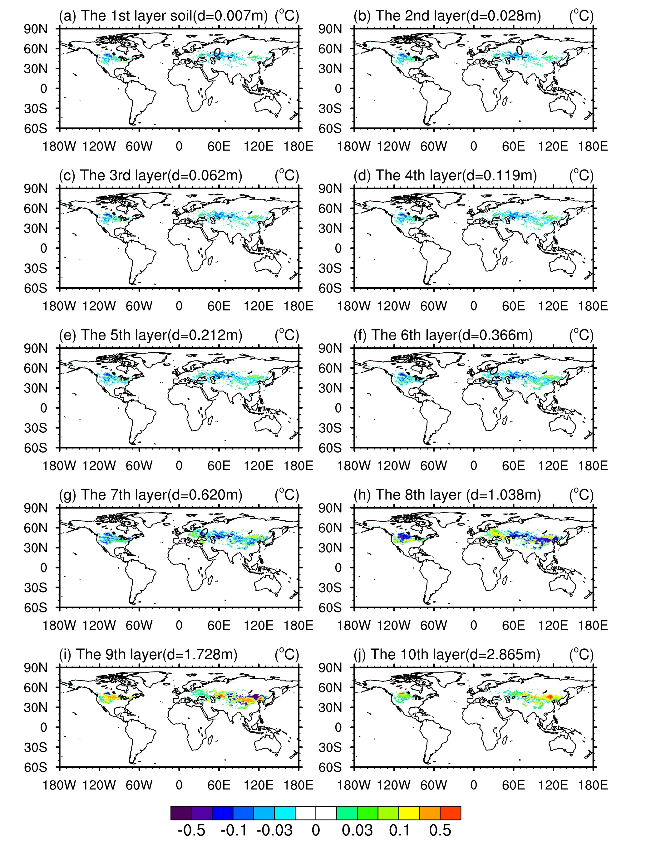
Fig.7.The difference between January soil temperature at different soil layers simulated by CoLM, which considers the dynamic change of soil freezing-thawing fronts, and the original land surface model CoLM in the seasonally frozen ground region.
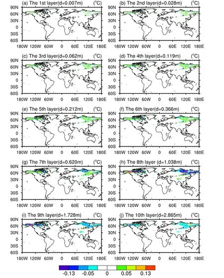
Fig.8.The difference between July soil temperature at different soil layers simulated by CoLM, which considers the dynamic change of soil freezing-thawing fronts, and the original land surface model, CoLM, in the permafrost region.
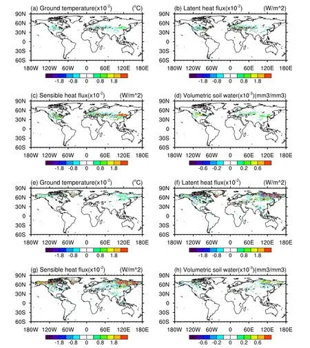
Fig.9.The differences in ground temperature, latent heat flux, sensible heat flux, and volumetric soil water in the seasonally frozen ground region and permafrost regions between a CoLM simulation that considers the dynamic change of soil freezing and thawing fronts, and the original land surface model, CoLM.
Accurate simulation of soil freezing and thawing fronts is significant for studying energy, hydrology, carbon and nitrogen cycles, and infrastructure construction in frozen ground.Although we can directly calculate freezing and thawing fronts by interpolating simulated original soil temperatures into fine soil layers, the subsequent interpolation of soil temperature may exhibit large fluctuations during autumn freezing and spring snowmelt periods when the soil temperature hovers around the freezing point (Yi et al.,2006; Gao et al., 2019).Stefan’s equation is a semi-empirical approach for successfully simulating the depths of soil freezing and thawing fronts (Fox, 1992; Li and Koike, 2003).Stefan’s equation requires only a few parameters to calculate the soil freezing and thawing fronts and has a simple form.Therefore, Stefan’s equation is widely used in various engineering construction applications on frozen ground.This method can simulate and predict the changes in soil freezing and thawing fronts more accurately.Stefan’s equation was developed with a multi-layer soil Stefan algorithm to calculate the depth of freezing and thawing fronts by Woo et al.(2004).The multi-layer soil Stefan algorithm can be coupled to a land surface model.Although Stefan’s equation can successfully simulate the depths of soil freezing and thawing fronts, its semi-empirical approach has limitations.The model assumes that all absorbed or released energy by the soil is used to transform soil water and ignores the sensible heat energy arising from temperature changes in the soil.Such an assumption can lead to simulation errors.Due to such considerations, further study is needed regarding the physical processes of freezing and thawing and in accurately simulating soil freezing and thawing fronts.
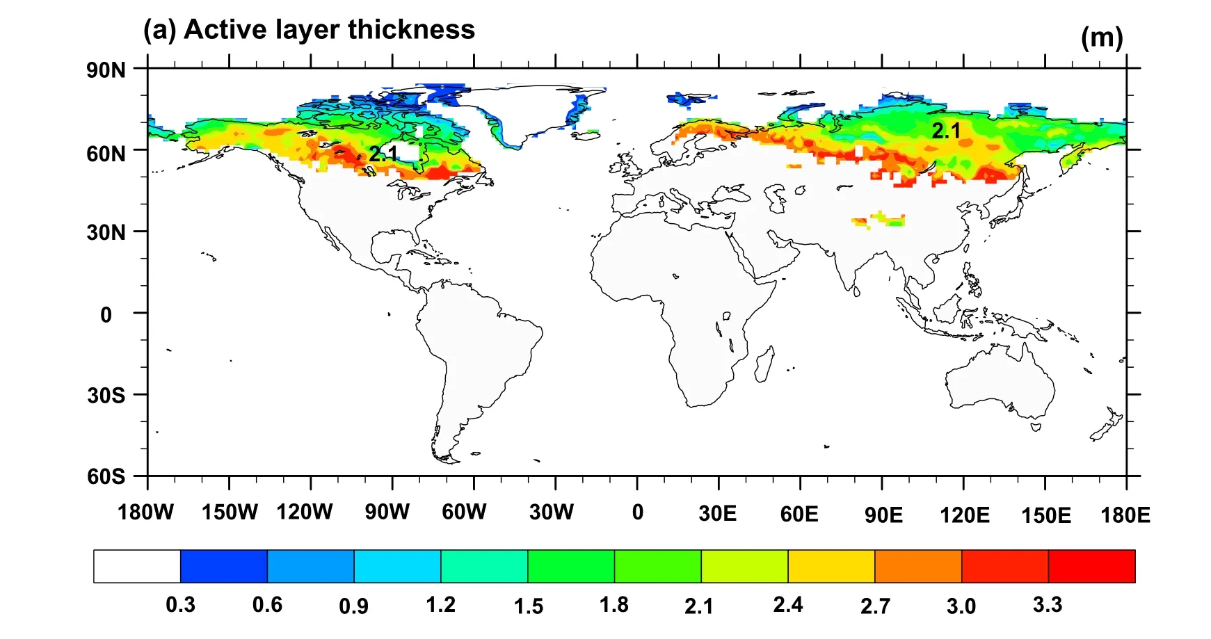
Fig.10.Spatial distribution of simulated active layer thickness by CAS-ESM from 1990 to 2000 in the permafrost region.
In this paper, the multi-layer soil Stefan algorithm for calculating freezing and thawing fronts was coupled to the land surface model (CoLM) to develop a land surface model that considers the change of soil freezing and thawing fronts.In the coupling process, the multi-layer soil Stefan algorithm that calculates freezing and thawing fronts was first coupled to the soil temperature calculation module in the land surface process model, CoLM, to simulate the change of soil freezing and thawing fronts.Then, the location information of the simulated soil freezing or thawing front was added to the original soil layer to update the soil layer and improve the ability to simulate the temperature of the thicker soil layer.Results show that the developed models could reproduce the soil freezing and thawing process and the dynamic change of freezing and thawing fronts.The regionally averaged value of active layer thickness in permafrost regions from 1990 to 2000 was 1.92 m.The regionally averaged trend value was 0.35 cm yr—1, and the active layer thickness increased yearly.The regionally averaged value of maximum freezing depth in seasonally frozen ground regions from 1990 to 2000 was 2.15 m, and the regionally averaged trend value was—0.48 cm yr—1.The maximum freezing depth decreased year by year.Our results indicate that climate change has had a significant effect on the active layer thickness of permafrost,and this finding has the potential to further our understanding of the responses of active layer thickness to climate change.
Acknowledgements.This work was jointly funded by the National Natural Science Foundation of China (Grant Nos.42205168, 41830967, and 42175163), the Youth Innovation Promotion Association CAS (2021073), and the National Key Scientific and Technological Infrastructure project “Earth System Science Numerical Simulator Facility”(EarthLab).
 Advances in Atmospheric Sciences2023年9期
- Advances in Atmospheric Sciences的其它文章
- The 17th Workshop on Antarctic Meteorology and Climate and 7th Year of Polar Prediction in the Southern Hemisphere Meeting
- Modulation of the Wind Field Structure of Initial Vortex on the Relationship between Tropical Cyclone Size and Intensity
- A Lagrangian Trajectory Analysis of Azimuthally Asymmetric Equivalent Potential Temperature in the Outer Core of Sheared Tropical Cyclones
- The Processes-Based Attributes of Four Major Surface Melting Events over the Antarctic Ross Ice Shelf
- Hybrid Seasonal Prediction of Meridional Temperature Gradient Associated with “Warm Arctic-Cold Eurasia”
- Enhanced Seasonal Predictability of Spring Soil Moisture over the Indo-China Peninsula for Eastern China Summer Precipitation under Non-ENSO Conditions