Hybrid Seasonal Prediction of Meridional Temperature Gradient Associated with “Warm Arctic-Cold Eurasia”

Tianbao XU, Zhicong YIN*,2,3, Xiaoqing MA, Yanyan HUANG,2,3, and Huijun WANG,2,3

1Key Laboratory of Meteorological Disaster, Ministry of Education / Joint International Research Laboratory of Climate and Environment Change (ILCEC) / Collaborative Innovation Center on Forecast and Evaluation of Meteorological Disasters (CIC-FEMD), Nanjing University of Information Science & Technology, Nanjing 210044, China

2Southern Marine Science and Engineering Guangdong Laboratory (Zhuhai), Zhuhai 519080, China

3Nansen-Zhu International Research Centre, Institute of Atmospheric Physics, Chinese Academy of Sciences,Beijing 100029, China

ABSTRACT The meridional gradient of surface air temperature associated with “Warm Arctic—Cold Eurasia”(GradTAE) is closely related to climate anomalies and weather extremes in the mid-low latitudes.However, the Climate Forecast System Version 2 (CFSv2) shows poor capability for GradTAE prediction.Based on the year-to-year increment approach, analysis using a hybrid seasonal prediction model for GradTAE in winter (HMAE) is conducted with observed September sea ice over the Barents—Kara Sea, October sea surface temperature over the North Atlantic, September soil moisture in southern North America, and CFSv2 forecasted winter sea ice over the Baffin Bay, Davis Strait, and Labrador Sea.HMAE demonstrates good capability for predicting GradTAE with a significant correlation coefficient of 0.84, and the percentage of the same sign is 88% in cross-validation during 1983-2015.HMAE also maintains high accuracy and robustness during independent predictions of 2016-20.Meanwhile, HMAE can predict the GradTAE in 2021 well as an experiment of routine operation.Moreover, well-predicted GradTAE is useful in the prediction of the large-scale pattern of “Warm Arctic—Cold Eurasia”and has potential to enhance the skill of surface air temperature occurrences in the east of China.

Key words: warm Arctic—cold Eurasia, year-to-year increment, climate prediction, sea ice, SST

1.Introduction

The warming trend in the Arctic and cooling in Eurasia are generally significant in wintertime (Xie et al., 2022).The “Warm Arctic—Cold Eurasia”(WACE) pattern has been well recognized as a dominant interannual variability in winter (Sung et al., 2018).The WACE pattern could contribute to the decrease in the large-scale meridional gradient of surface air temperature (SAT) in the mid-high latitudes and reduce atmospheric baroclinicity (Cohen et al., 2014).As a result, more cold air mass can be transported to the mid-low latitudes compared to that solely caused by Arctic warming (Zhang et al., 2021).The intense snowfall event that occurred in central eastern China during January 2018(Sun et al., 2019) and the record-breaking cold waves in eastern China in 2020/21 (Zhang et al., 2021) both were influenced by the reduced meridional gradient of SAT associated with the WACE pattern (GradTAE).Therefore, it is necessary and meaningful to predict the GradTAEin winter.

Several previous studies have investigated the effect of Arctic sea ice on the mid-latitude climate (Wang and Liu,2016; Cheung et al., 2018).With global warming and particularly the loss of sea ice in the Barents—Kara Sea, Arctic amplification is becoming more prominent and has resulted in a stronger connection between the Arctic and the mid-high latitudes of the Northern Hemisphere (Vihma, 2014).Arctic warming may reduce the meridional gradient of SAT and weaken the prevailing westerlies, which is favorable for midlatitude Eurasia to become cool (Liu et al., 2012).The sea ice decrease in autumn can also lead to more frequent formation of blocking high pressure in the Arctic—Eurasia region,which is conducive to extreme cold events in the midlatitudes of Eurasia (Mori et al., 2014; Zhang et al., 2022).Ocean variability can also affect SAT in the Arctic and Eurasia.Variations in sea surface temperature (SST) outside the Arctic are a long-term driving force for tropospheric warming over the Arctic, because of the increased heat transport to the polar region (Screen et al., 2012).The SST anomaly in the North Atlantic can trigger Rossby waves, which are conducive to the formation of the WACE pattern (Jung et al., 2017).Meanwhile, soil moisture (SoM) has the capability to remember aberrant change signals from the atmosphere, which can greatly influence the temporal evolution of climate (Chen and Zhou, 2013).Seasonal anomalies of SoM have considerable influences on seasonal fluctuations of the atmosphere,particularly SAT (Berg et al., 2014).

In addition to those preceding signals, regional thermal processes and current atmospheric circulations are also crucial for climate prediction.Based on this fact, hybrid climate prediction models can be developed by combining current predictors derived from general circulation model outputs with preceding signals obtained from observational data to increase the prediction accuracy (Ji and Fan, 2019).Currently, various approaches for SAT prediction in the Arctic or Eurasia in winter have been developed (Yoo et al., 2018;Chang et al., 2021).However, methods to predict the GradTAEare still less than sufficient.Furthermore, most of the climate models show limited skill for the simulation of the SAT relationship between the Arctic and Eurasia (Jung et al., 2020),and climate prediction in the mid-high latitudes has always been a challenging issue (Wang et al., 2022).Thus, establishing a dynamic—statistical hybrid prediction model to strengthen the prediction skill of the GradTAEis necessary.

Compared with traditional approaches, the year-to-year increment approach can better acquire the interdecadal component by utilizing the observed values of the previous year and can also amplify the prediction signals (Fan et al.,2008).This approach has been applied to improve the prediction skill for summer temperature in Northeast China (Fan and Wang, 2010), the winter North Atlantic Oscillation(Tian and Fan, 2015), and winter haze days and PM2.5concentration in North China (Yin and Wang, 2017; Yin et al.,2022a, b).Furthermore, the large-scale circulation over the Arctic and Eurasia, e.g., the Siberian High (Yang and Fan,2021) in winter, has been successfully predicted using the year-to-year increment approach.Therefore it is feasible that the year-to-year increment approach might be utilized to predict the GradTAE.

The remainder of this paper is organized as follows.Section 2 describes the datasets and methods used.The features of the GradTAEand the performance of the Climate Forecast System Version 2 (CFSv2) for the prediction of the GradTAEare examined in section 3.Predictors and relevant physical processes are discussed in section 4.In section 5, the prediction model is constructed and its performance is verified.A summary and further discussion are presented in section 6.

2.Datasets and methods

The fifth-generation reanalysis product (ERA5) produced by the European Center for Medium Range Weather Forecasts is employed in this study (Hersbach et al., 2020).The dataset includes daily SAT, SST, SoM (0-7 cm), snowfall, zonal and meridional winds, surface sensible and latent heat fluxes, mean sea level pressure (SLP), geopotential height at different vertical levels on global 1°×1° grids for the period 1982-2021.The surface heat flux (SHF) is defined as the sum of surface sensible and latent heat fluxes,which is positive downward.The monthly sea ice concentration (SIC) dataset with a spatial resolution of 1° × 1° is provided by the Met Office Hadley Centre (Rayner et al., 2003).The winter SAT and SIC data used here are also produced by CFSv2, which is an atmosphere—ocean—sea-ice—land model system (Saha et al., 2014) that is used for both retrospective forecast experiments (1982-2010) and operational forecasts (since 2011).The winter CFSv2 dataset used in this study is released in November (one month in advance)with a 1° × 1° resolution for the period 1982-2021.

Empirical orthogonal function (EOF) analysis is conducted to separate and obtain the main temporal and spatial patterns of variables (North et al., 1982).Horizontal wave activity fluxes (WAF) are computed to analyze the propagation of Rossby waves based on the equations proposed by Plumb (1985):

where p is the pressure, u and v represent zonal and meridional winds,Фis the geopotential height,Ωis the earth’s rotation rate,αis the earth’s radius, andφandλare the latitude and longitude, respectively.

The year-to-year increment approach is proposed to improve the climate prediction skill.In this approach, the predicted object is the difference between the current year and the previous year (DY).The final prediction is generated by combining the predicted DY with the observed predictand from the previous year, i.e., DY = Yt-Yt-1.The “l(fā)eave-oneout cross-validation”method (Michaelsen, 1987), which deletes one year of the variable from its time series and derives a prediction model from the remaining series, is used to verify the prediction skill of the model.In this study,we perform the cross-validation of results over the period 1983-2015 and conduct independent prediction for the period 2016-20.An experiment of routine operation for 2021 is also conducted.Using the leave-one-out cross-validation method, root-mean-square error (RMSE), mean absolute error (MAE), correlation coefficient (CC), and the percentage of the same sign (PSS) are calculated.The winter season is defined as December in the current year and January to February in the next year.From 1 December to 14 January and 15 January to 28 February are defined as the early and late winter, respectively.

3.The GradTAE changes and prediction skill of CFSv2

The linear trend of SAT in winter demonstrates warming in the Arctic and cooling in Eurasia during 1982-2020 (Figure not shown), and this trend is more obvious from 1996 to 2012 (Fig.1a) (Jin et al., 2020).The SAT difference between the Barents—Kara Sea (65°-85°N, 30°-90°E) and Eurasia (40°-60°N, 60°-120°E) (former minus later) is defined as the GradTAE, which is used to demonstrate the SAT difference between the two areas and reflect the meridional gradient.The GradTAEand the local SAT gradient in the transition region of Arctic—Eurasia (60°-65°N, 30°-120°E) exhibit a significant negative correlation [Fig.S1 in the electronic supplementary material (ESM)], and the CC between them is -0.81 (exceeding the 99% confidence level).This shows that the GradTAEcan reflect not only the average SAT gradient of the two centers, but also the local SAT gradient between them.The observed GradTAEshows a downward trend during 1982-95 and an obvious upward trend during 1996-2012 (Fig.1b).Over the period of 2013-20, the GradTAEchanged steadily (Blackport and Screen, 2020).Meanwhile, based on previous studies, the second EOF mode of winter SAT anomalies over the region(20°-90°N, 0°-180°E) is characterized by the WACE pattern(Fig.S2 in the ESM), and the corresponding time series is defined as PWACE(Mori et al., 2014), which can adequately depict the interannual variability characteristics of the WACE pattern (Sung et al., 2018).With a high CC of 0.97(exceeding the 99% confidence level), PWACEand the Grad-TAEare significantly correlated (Fig.1b).Therefore, the prediction of the GradTAEhas great indicative meaning for the interannual variability of the WACE pattern.

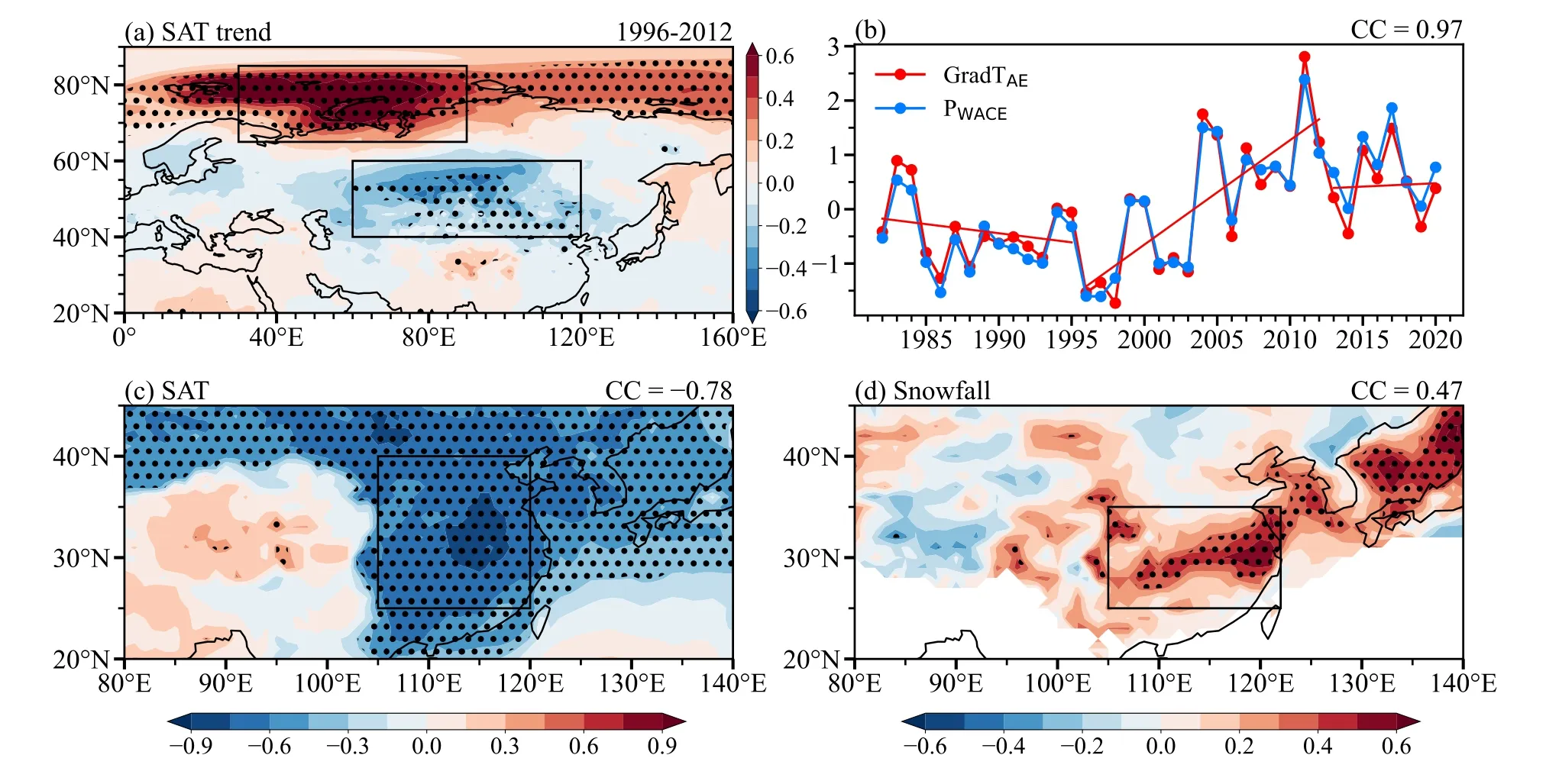
Fig.1.(a) Linear trend of DJF SAT during 1996-2012.The black dots indicate the linear trend exceeding the 95%confidence level.The black boxes represent the centers of the GradTAE.(b) Variations in the normalized GradTAE (red) and PWACE (blue) from 1982 to 2020.The solid lines represent the linear trend.Correlation coefficients of the GradTAE with(c) SAT and (d) snowfall after detrending in the winters of 1982-2020.The black dots indicate CCs exceeding the 95%confidence level.The black boxes are the east of China and Yangtze River Delta regions.

In addition, taking the early 21st century as the dividing line, most of the negative values of the GradTAEappear in the former period and most of the positive values occur in the latter period (Fig.1b).The lowest and highest values of the index appear in 1988 and 2011, respectively, corresponding to the times when the Arctic SAT is lower and higher than that in Eurasia, respectively (Fig.S3 in the ESM).As the GradTAEreached its highest value in 2011, the averaged winter SAT over China reached its lowest value since 1986 in 2011 (Sun et al., 2012).In the winter of 2004, two largescale strong cold wave processes occurred in China (Ma et al., 2008), and the GradTAEin this year was also significantly higher.It can be seen that the GradTAEis closely related to weather and climate in the mid-low latitudes.In order to further explore the relationship between the GradTAEand climate anomalies in the mid-low latitudes, the relationships between SAT, snowfall, and the GradTAEare discussed.The GradTAEis highly associated with SAT in the east of China (SATEC; 25°-40°N, 105°-120°E) with a CC value of-0.78 (exceeding the 99% confidence level) between the detrended GradTAEand SATECfrom 1982 to 2020 (Fig.1c).The GradTAEis also significantly and positively correlated(with a CC of 0.47 that exceeds the 99% confidence level)with snowfall in the Yangtze River Delta region (25°-35°N,105°-122°E) (Fig.1d).It can be seen that the influence of the GradTAEis not just limited to the Arctic—Eurasia region,but also extends to the mid-low latitudes.

The CFSv2 has been documented as a reliable tool for seasonal forecasting with high accuracy in SAT predictions(Saha et al., 2014).Therefore, CFSv2 predictions in November are used to evaluate the prediction skill of the winter Grad-TAEand GradTAE-DY with a lead time of one month.The CC of the GradTAEbetween the observations and CFSv2 outputs is 0.58 during 1982-2020 (Fig.2a), and the CC is 0.48 after detrending.Differences between observations and CFSv2 outputs are also measured by RMSE and MAE,whose values are 3.4°C and 2.57°C, respectively.The differences between observations and CFSv2 predictions are obvious, which indicates that CFSv2 cannot accurately describe the specific interannual changes of the GradTAE.In addition,an obvious underestimation of the GradTAEtrend is also found in CFSv2 outputs (Fig.2a).In particular, the biases of CFSv2 outputs are ever-increasing after 2000, and CFSv2 cannot reproduce the positive values of the GradTAE.CFSv2 also has no skillful prediction effect for the maximum value in 2011.The observed GradTAE-DY exhibits a distinct feature of biennial oscillation, implying that it is more predictable than the original GradTAE(Fig.2b).From 1996 to 2020, GradTAE-DY first varied substantially and then maintained a large amplitude, indicating that it can be better predicted after the mid-1990s.The CC of GradTAE-DY between observations and CFSv2 predictions is 0.37, which indicates that CFSv2 cannot reproduce the characteristics of the GradTAE-DY well (Fig.2b).As a consequence, CFSv2 still has a lot of room for improvement for its prediction skill of the GradTAE.Under these circumstances, building prediction models with external forcing drivers might be a practicable route to obtain improved seasonal prediction of the GradTAE.

4.Predictors and associated mechanisms

4.1.SIC over the Barents-Kara Sea

The autumn Arctic sea ice might induce atmospheric responses and subsequently influence winter climate in the Arctic—Eurasia region (Mori et al., 2014; Zhang and Screen,2021).The preceding September SIC-DY over the Barents—Kara Sea is negatively correlated with the GradTAE-DY.The area-averaged (75.5°-82.5°N, 20.5°-90.5°E; the green box in Fig.3a) SIC-DY in September is calculated and defined asx1, and the CC betweenx1and the GradTAE-DY is -0.62 (exceeding the 99% confidence level) during 1983-2015 (Fig.4, Table S1 in the ESM).

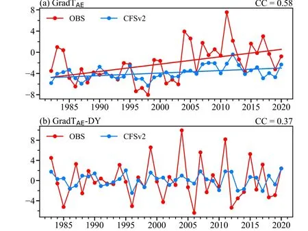
Fig.2.Variations of the observed (red) and CFSv2-predicted (blue):(a) GradTAE from 1982 to 2020 and (b) GradTAE-DY from 1983 to 2020.The solid lines in (a) represent the linear trends.

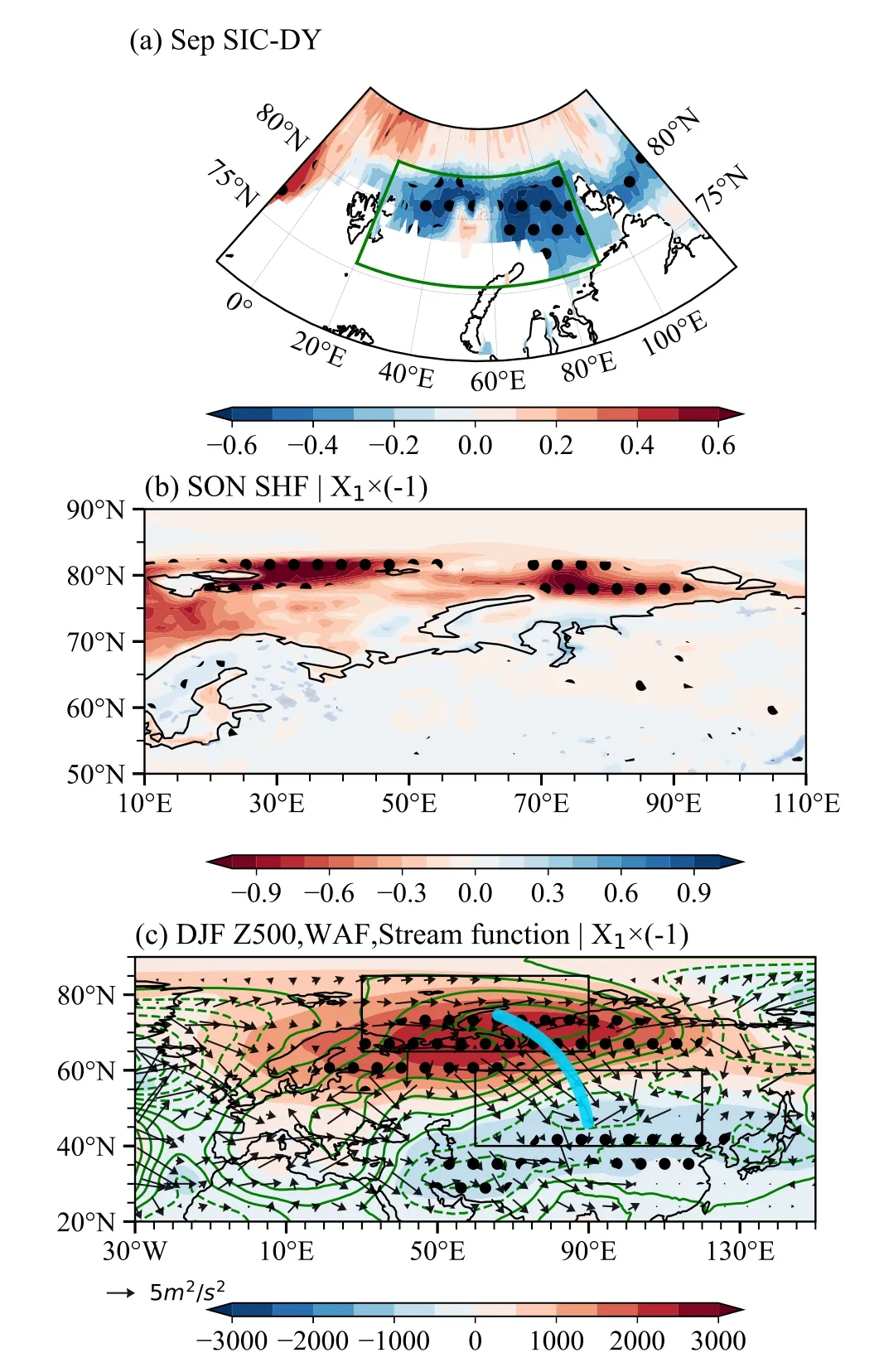
Fig.3.(a) Correlation coefficient map between the GradTAEDY and Sep SIC-DY during 1983-2015.The black dots indicate CCs exceeding the 95% confidence level.The sea ice areainthe greenboxisaveragedas the x1.Regressionsof variableson negative x1during1983-2015:(b)SON SHF-DY(shadings; units: 107 W m-2); (c) DJF Z500-DY (shadings;units: gpm), WAF (vectors; units: m2 s-2), and quasigeostrophic stream function (contours; units: 106 m2 s-1)at 500 hPa.The black boxes in (c) represent the centers of the GradTAE.The black dots indicate regression coefficients exceeding the 95% confidence level.

The decrease in September SIC-DY over the Barents—Kara Sea could influence local upward surface adiabatic heating anomalies in autumn (Fig.3b).The heat flux anomaly corresponding to reduced sea ice in September could trigger atmospheric responses.In the middle troposphere, the anomalous Rossby WAF can propagate from the Barents—Kara Sea (anticyclonic) to the middle latitudes of Eurasia(cyclonic) in winter (Fig.3c), leading to a stronger than normal East Asian trough and Ural high.Such changes in the atmospheric circulation are favorable for the occurrence of cold conditions in the lower latitudes of Eurasia (Wang and Jiang, 2004; Cheung et al., 2013).Meanwhile, the predominant midlatitude westerlies are weakened, while the northerlies that promote the southward invasion of cold air are enhanced (He and Wang, 2012).Under this condition, more cold and dense air mass accumulates in the middle troposphere.Anomalous divergence develops in the lower troposphere as a consequence of intense descending motion and a cooling surface.Moreover, the sea ice decrease in the preceding September leads to an increase in heat absorbed by the ocean, and this increased heat is later released to the atmosphere and contributes to an SAT increase in the Arctic (Xie et al., 2022).Eventually, the SAT difference between the Arctic and Eurasia becomes larger and affects GradTAEchanges.

4.2.SST over the North Atlantic

North Atlantic SST has significant influences on climate system variation in Eurasia (Liu et al., 2014).The GradTAEDY is significantly and negatively correlated with SST-DY in the preceding October over the region of the North Atlantic (52°-70°N, 10°-65°W; the green box in Fig.5a).Here, we usex2to denote the average SST-DY over this region, and the CC betweenx2and the GradTAE-DY time series is -0.64 (exceeding the 99% confidence level) from 1983 to 2015 (Fig.4, Table S1).

Negative SST-DY in the North Atlantic could trigger cyclonic anomalies over the Labrador Sea and the anomalous Rossby WAF can propagate through two branches to Eurasia.The northward branch of the Rossby waves propagate to the Barents—Kara Sea and then to Eurasia (Fig.5b) (Sato et al., 2014; Jung et al., 2017).The southward branch of the Rossby waves can enhance the cyclone anomaly in the eastern Atlantic and propagate northward to the Arctic—Eurasia region.It is similar to the Scandinavia pattern (Barnston and Livezey, 1987), which consists of three circulation centers over Scandinavia, Europe, and Mongolia, respectively.Anticyclonic and cyclonic anomalies in the middle troposphere are found over the Barents—Kara Sea and the middle latitudes of Eurasia, respectively, which lead to SAT differences between the two regions.Meanwhile, the anticyclonic circulation anomaly over the Barents—Kara Sea also tends to transport warm air from the midlatitudes to the Arctic along its western flank, which is favorable for Arctic warming (Xie et al., 2022).In summary, the Rossby waves triggered by North Atlantic SST lead to warming of the Arctic and cooling of Eurasia, and the meridional SAT difference between the Arctic and Eurasia is subsequently changed.

4.3.Soil moisture in southern North America

In addition to the signal from the ocean, another crucial factor for seasonal prediction is SoM, and the SoM memory of climate anomalies plays an important role in the influence on climate (Koster et al., 2010; Chen and Zhou, 2013).We examine the relationship between autumn SoM-DY and the GradTAE-DY in southern North America (20°-50°N, 80°-120°W; the green box in Fig.6a).It is found that September SoM-DY is negatively correlated with the variation of the GradTAE-DY.x3is defined as the area-averaged SoM-DY,which is significantly and negatively correlated with the Grad-TAE-DY (CC = -0.63; exceeding the 99% confidence level)from 1983 to 2015 (Fig.4, Table S1).

Fig.4.Temporal variations of the normalized GradTAE-DY and predictors(x1,x2,x3 and x4) during 1983-2015.The CCs indicate the correlation coefficients between the GradTAE-DY and predictors.

The abnormally low SoM could trigger anticyclonic anomalies at 500 hPa over eastern North America in September (Fig.6b).Likewise, adjacent cyclones and anticyclones occur over the northern Atlantic and the Barents—Kara Sea.The anticyclone over the Barents—Kara Sea can lead to the reduction of SIC-DY through the downward heat flux(Fig.6cd).It also has the same effect on October SIC-DY (figure not shown).The influence of soil moisture on the reduction of sea ice can trigger an anticyclone over the Barents—Kara Sea and a cyclone over Eurasia in winter (Fig.6e),which leads to changes in the SAT gradient between the Arctic and Eurasia.

4.4.Winter SIC from CFSv2 outputs

Winter climate factors also have important influences on the SAT gradient between the Arctic and Eurasia.Therefore, we attempt to explore a current climate factor from the CFSv2 as a predictor.Based on CFSv2 outputs, the GradTAE-DY and SIC-DY in winter over the region (50°-80°N, 45°-90°W; the green box in Fig.7a) around Baffin Bay, Davis Strait, and the Labrador Sea are significantly and positively correlated.Previous studies have revealed that the increase of sea ice over this region in winter is closely related to the climate anomalies over Eurasia (Wu et al., 2013) and can lead to quasi-stationary Greenland blocking events with strong cold anomalies appearing over Eurasia(Chen and Luo, 2017, 2021), which can expand the SAT gradient over the Arctic—Eurasia region.Therefore, the average SIC-DY over this region is referred to asx4(Table S1).The winter SIC-DY from observed data also shows a significant negative correlation with the GradTAE-DY in Baffin Bay,Davis Strait, and the Labrador Sea (Fig.7b).By comparing the CFSv2 outputs with the observed data (Fig.7c), it is found that CFSv2 can predict the winter SIC-DY well.The CC betweenx4derived from observation and that from CFSv2 data is 0.7 (exceeding the 99% confidence level)(Fig.7d), and the CC betweenx4and the GradTAE-DY time series is 0.43 (exceeding the 95% confidence level) during 1983-2015 (Fig.4, Table S1).Therefore, the current SIC can be used as one of the predictors.

5.Prediction models and validation

Based on the physical mechanisms discussed above,four normalized predictors (x1-x4) are used to develop the hybrid seasonal prediction model using the year-to-year increment approach for the GradTAE-DY (HMAE).These predictors contain different extrinsic forcing factors to ensure efficient and abundant signals can be involved as much as possible.The multicollinearity problem is insignificant since the largest variance inflation factor is less than 2.14.The HMAEis trained with the external forcing factors and is expressed as follows:GradTAE-DY= -0.39x1-0.33x2-0.35x3+0.16x4.In this section, the hybrid seasonal prediction models are established and validated in detail.

Fig.5.(a) Correlation coefficient map between the GradTAE-DY and Oct SST-DY during 1983-2015.The black dots indicate CCs exceeding the 95% confidence level.(b) Regressions of DJF Z500-DY (shadings; units: gpm), WAF (vectors; units: m2 s-2), and quasigeostrophic streamfunction (contours;units:106m2 s-1)at500hPaon negativex2 during1983-2015.The greenbox representsthe centersof x2,andthe blackboxesrepresent the centers of the GradTAE.The black dots indicate regression coefficients exceeding the 95%confidence level.

The prediction models are evaluated by leave-one-out cross-validation for prediction over 1983-2015 and independent prediction for prediction over 2016-20.For the prediction effect of the GradTAE-DY during 1983-2015, the CC between the observed and fitted GradTAE-DY values is 0.79 during 1983-2015, which exceeds the 99% confidence level(Table 1, Fig.8a).The RMSE, MAE, and PSS between the fitted and observed GradTAE-DY are 2.38°C, 1.82°C, and 73%, respectively.The HMAEcan reproduce the variation of the GradTAE-DY and capture its extreme value in 2011.Furthermore, the large amplitudes after 2000 are simulated well.

To obtain the climate anomalies, the final GradTAEprediction is produced by adding the predicted GradTAE-DY obtained from the HMAEto the observed GradTAEin the previous year (Fig.8b).The PSS reaches 88%, which is 15%higher than that for the GradTAE-DY (Table 1).This result confirms that the model can better predict the GradTAEcompared to the prediction of the GradTAE-DY.In the leave-oneout cross validation for the GradTAE, the CC between the observations and predictions is 0.84 (exceeding the 99%confidence level) during 1983-2015, indicating that the linear trend removed by the DY approach is reintroduced successfully.After detrending, the CC is 0.81, which also exceeds the 99% confidence level, suggesting that the HMAEalso reflects the annual variation well.Compared with CFSv2,the prediction result of the HMAEis significantly improved,with the CC increasing by 29%, RMSE decreasing by 28%,and MAE decreasing by 26% for the period 1983-2015.For the independent prediction results of the HMAEfor 2016 to 2020, the biases (the predicted value minus the measurement) of the predicted GradTAEare -0.83°C, -1.94°C,5.2°C, -2.24°C, and 1.52°C, respectively.Although there is a large bias in the prediction for 2018, the interannual variation can be predicted well.For trends in various periods, the downward trend during 1983-95, the upward trend during 1996-2012, and the steady trend of the GradTAEduring 2013-20 can also be predicted well (Fig.8b).Thus, the linear trend and the interannual variation of the GradTAEare both simulated well by the HMAE.

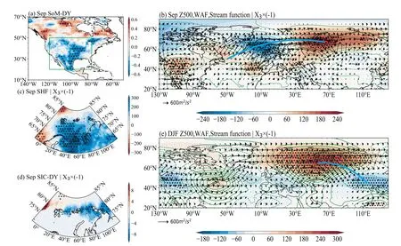
Fig.6.(a) Correlation coefficient map between the GradTAE-DY and Sep SoM-DY during 1983-2015.The black dots indicate CCs exceeding the 95% confidence level.The soil moisture values in the green box are averaged as x3.Regressions of variables on negative x3 during 1983-2015: (b) Sep Z500-DY (shadings; units: 102 gpm), the associated horizontal WAF(vectors; units: m2 s-2), and quasigeostrophic stream function (contours; units: 106 m2 s-1) at 500 hPa; (c) Sep SHF-DY(shadings; units: W m-2); (d) Sep SIC-DY (shadings); (e) the same as (b) but for DJF.The black dots indicate regression coefficients exceeding the 95% confidence level.

A hybrid prediction model is also established using the same predictors used in the HMAEbut in an anomaly form.The CC and CC after detrending between the anomaly form model-predicted and observed GradTAEare 0.72 and 0.65,respectively (figure not shown).Although the anomaly form model yields a lower prediction skill than the HMAE, it still maintains prediction ability to a certain degree.This indicates that the selected predictors are stable.Meanwhile, considering the excellent performance of the HMAEin predicting the GradTAE, and the high correlation between the GradTAEand PWACE(Fig.1b), a new model is applied to predict PWACEusing the same predictors of the HMAE(HMWACE).The cross-validation and performance of independent prediction are shown in Fig.S4 (in the ESM) and Table 1.For the effect of PWACEprediction during 1983-2015, leave-one-out cross-validation indicates that the CC between the observed and fitted PWACEis 0.87, which exceeds the 99% confidence level.However, the CC between the prediction result of CFSv2 and observations is only 0.39.Note that the HMWACEmodel shows a better prediction skill for PWACEthan CFSv2.The RMSE, MAE, and PSS between fitted and observed PWACEare 0.59%, 0.44%, and 82%, respectively(Table 1).Compared with CFSv2, RMSE and MAE decreased by 62% and 66%, respectively, and PSS increased by 43%.The CC between observations and HMWACEpredictions of PWACEafter detrending is 0.83,which is 0.4 higher than that predicted by CFSv2.For the independent prediction results for 2016 to 2020, the biases of the predicted PWACEare less than 1.0 in all five years except 2018.This result shows that the factors can not only predict the GradTAEwell, but also can be used to predict the interannual variability of the WACE pattern.

6.Conclusions and discussion

The need for skillful prediction of the meridional gradient of SAT associated with the WACE pattern in winter has been continually growing.In this work, four climate factors are used to build a hybrid seasonal prediction model using the year-to-year increment approach.The GradTAE-DY is treated as the predictand, and the observed September SIC over the Barents—Kara Sea, October SST over the North Atlantic, September SoM in southern North America, and CFSv2 winter SIC over Baffin Bay, Davis Strait, and the Labrador Sea are selected as the predictors.The prediction skills of the prediction models are examined by applying the leave-one-out cross-validation method for the period 1983-2015 and independent prediction for the period 2016-20.

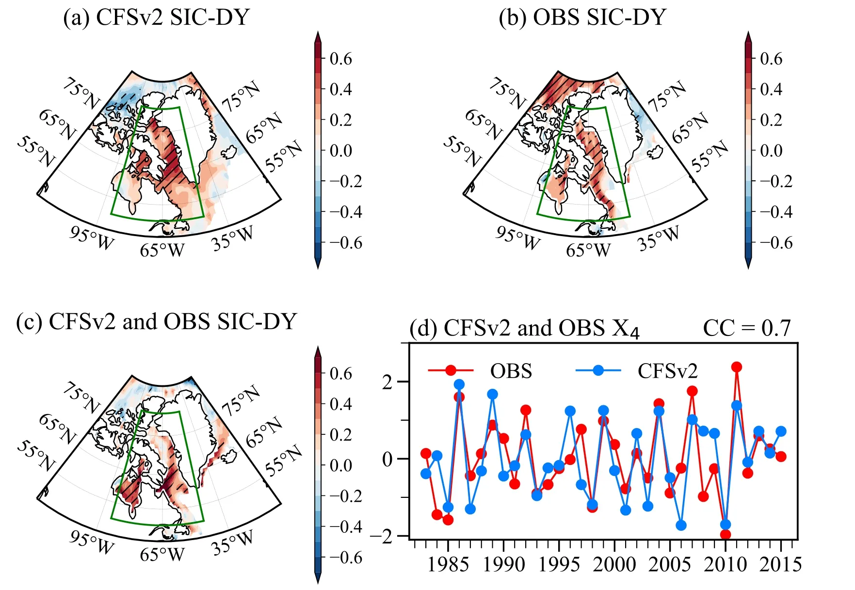
Fig.7.Correlation coefficient map between the GradTAE-DY and DJF SIC-DY based on (a) CFSv2 and (b)observeddata during1983-2015.The CFSv2 SIC-DYinthegreenboxis averagedasx4.(c)Correlation coefficientmapbetween theDJFSIC-DYof CFSv2outputsand observation.Theblack slashes indicate CCs exceeding the 90% confidence level.(d) The temporal variation of normalized x4 based on CFSv2 outputs (blue) and observation (red).

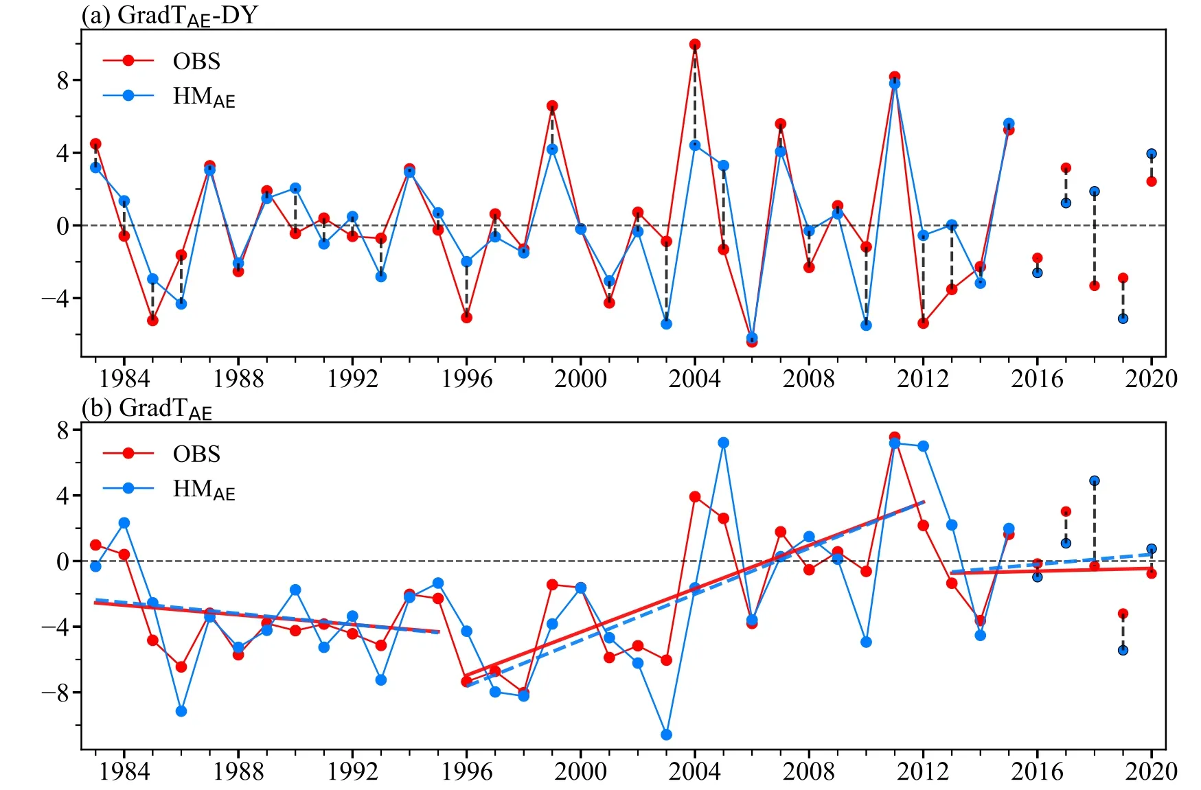
Fig.8.Temporal variations of (a) the GradTAE-DY and (b) GradTAE: observed (red), HMAE-predicted (blue).Leave-one-out cross-validation of prediction results by the HMAE are from 1983 to 2015, and independent prediction results by the HMAE are from 2016 to 2020.The solid and dashed straight lines represent the linear trends.

For the HMAE, the PSS and CC between observations and the predicted GradTAEare 0.84 and 88%, respectively.Furthermore, the interannual variability, the extreme values,and the significant trend in various periods are successfully captured.The independent predictions for 2016-20 have shown good prediction results, except for 2018, with a bias of about 2°C.The necessity of each predictor is further studied.Whenx1orx3is removed, the prediction effect of the model decreases significantly.Whenx2orx4is removed,the prediction effect of the model decreases slightly (Table S2).If the CFSv2 outputted predictor in winter is excluded,the independent forecast effect will become worse, especially in 2017 (figure not shown).At the same time,x1andx2have a robust relationship with the predictand, whilex3andx4have a growing relationship with the predictand (Fig.S5 in the ESM).Therefore, the four prediction factors are indispensable.Meanwhile, a new model is applied to predict PWACEusing the same predictors of the HMAE.The CC between model predictions and observations for 1983-2015 is 0.87.The independent prediction also yields good results for 2016-20.This result indicates that the factors can not only predict the GradTAEwell, but can also be used to predict interannual variation of the WACE pattern.At the same time, through the training of prediction factors from 1983 to 2020, an experiment of routine operation is conducted to predict the GradTAEin 2021 (figure not shown).With a bias close to zero, the HMAEmodel can perfectly predict the GradTAEin 2021.

Although the skillful hybrid seasonal prediction of the GradTAEdeveloped in this work is useful for making seasonal predictions, the underlying physical mechanisms of the climate predictors have not been fully understood, and further research is necessary.Recently, the obvious subseasonal variation of winter SAT has attracted extensive attention (Wei et al., 2021; Yang and Fan, 2022).Can SAT changes on the subseasonal time scale lead to bias in seasonal prediction? The annual bias of the HMAE-predicted GradTAEand difference in the GradTAEbetween early and late winter are shown in Fig.9.There are obvious interdecadal differences in the CC between them.The CC is 0.09 from 1983 to 1999, but the value reaches 0.50 above the 95% confidence level from 2000 to 2020 (Fig.9).The 21-year sliding correlation between them also shows a weak (high) correlation in the former (latter) period.When not considering the huge subseasonal changes in 1983 and 1984 in the former period, the variances of the difference in the GradTAEbetween early and late winter in the latter period is double that of the former period.The high frequency of subseasonal phase reversal between the WACE and “Cold Arctic—Warm Eurasia”(CAWE) patterns usually co-occurred with a weak seasonal WACE trend, and the subseasonal WACE/CAWE patterns maintained comparable intensity with those from 1996 to 2011 in recent years (Yin et al., 2023).Therefore, the frequent large subseasonal differences in the recent 20 years may be one of the factors that affect the prediction skill of the HMAEmodel.

As the prediction effect in 2018 is the worst in the independent prediction by the HMAE, the situation in 2018 is analyzed separately.In the early winter, SAT anomalies were obviously positive in the Arctic and negative in Eurasia (Fig.S6a in the ESM), and the GradTAEwas 3.87°C.In the latewinter, however, the positive anomalies in the Arctic turned to be negative, while the negative anomalies in Eurasia became weaker (Fig.S6b).As a result, the GradTAEchanged to -4.39°C.Therefore, the subseasonal large change of the GradTAEin the winter of 2018 may influence the performance of the model.We plan to consider other predictors related to subseasonal changes and investigate possible physical processes behind their correlations with the winter GradTAEin future work.

Table 1.RMSE, MAE, PSS, CC, and CC after detrending between predictions and observations from 1983 to 2015.The results are obtained by leave-one-out cross-validation.

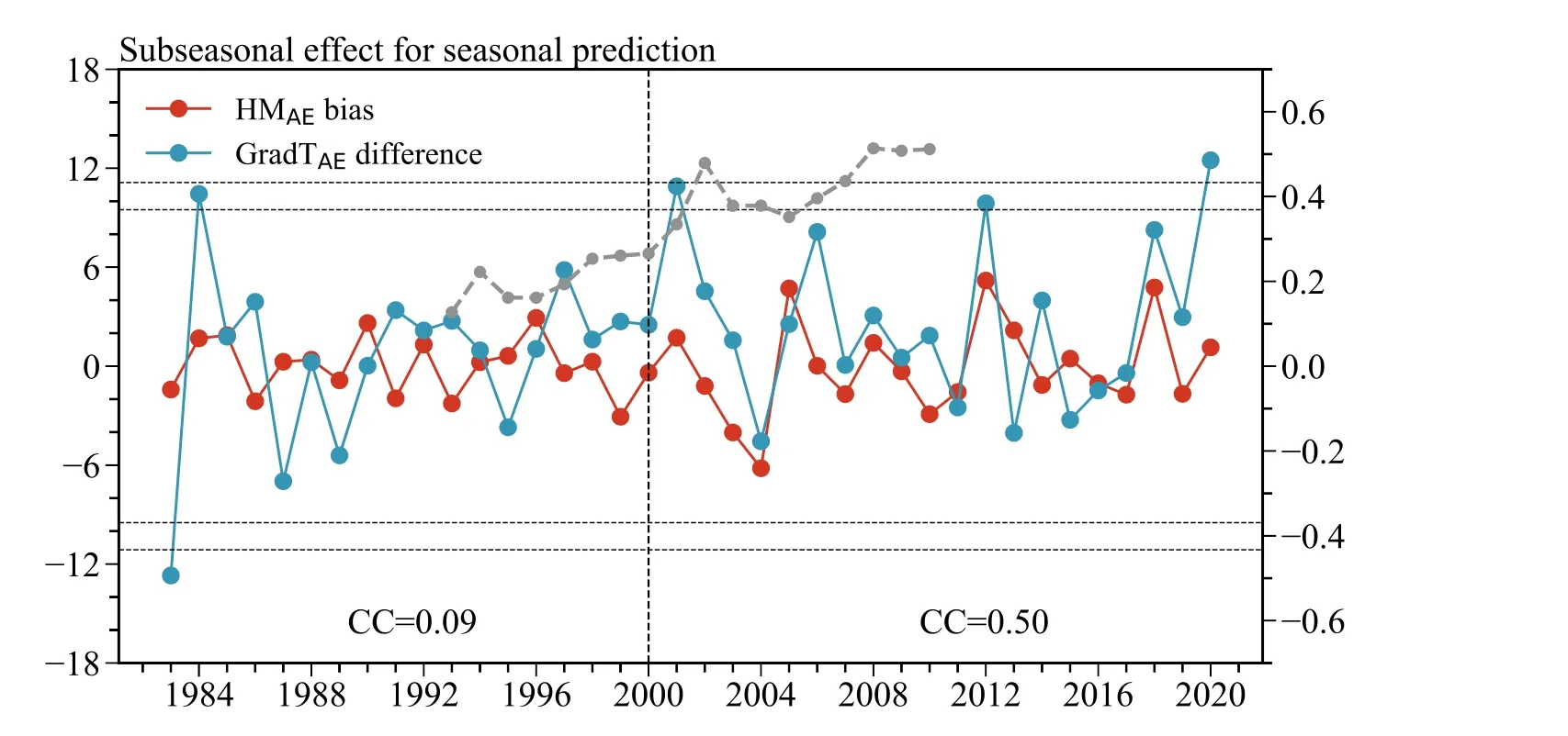
Fig.9.Temporal variations of annual bias of the HMAE-predicted GradTAE (red) and difference in the GradTAE (blue) between early and late winter.The correlation coefficients between them in 1983-99 and 2000-20 are given in the figure, respectively.The 21-year sliding correlation coefficients between them during the period of 1983—2020 (gray).The horizontal dashed lines indicate the 95% and 99% confidence levels, respectively.

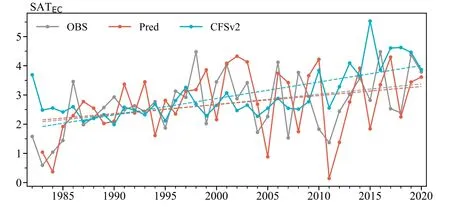
Fig.10.Variations of observed (gray) and CFSv2 (blue) SATEC from 1982 to 2020 and predicted SATEC (red) from 1983 to 2020.The predicted SATEC is produced by the prediction model that is trained by the HMAE-predicted GradTAE-DY and CFSv2-predicted SATEC-DY.The dashed straight lines represent the linear trends of observed and CFSv2 SATEC as well as predicted SATEC from 1983 to 2020.The results are based on leave-one-out cross-validation.

Cumulative evidence suggests that severe cold air outbreaks in the east of China have become more significant and frequent in the context of global warming (Luo et al.,2020).For example, the El Ni?o-Southern Oscillation(Zhou et al., 2007, 2009) and the connection between Ural—Siberian blocking and the East Asian winter monsoon(Cheung et al., 2012) may be reasons for the cooling in the east of China.However, the prediction skill of CFSv2 for the SATECis quite limited during 1983-2020 [CC = 0.32(0.02) before (after) detrending; Fig.10].Note that the Grad-TAEis highly associated with SAT in the east of China(Fig.1c).In order to test whether the GradTAEpredicted by the HMAEis helpful for improving the prediction skill of SATEC, the GradTAE-DY predicted by the HMAEmodel(leave-one-out cross-validation prediction results during 1983-2020) and the SATEC-DY output by CFSv2 are used as predictors to establish a prediction model for the SATEC(Fig.10).The CC between observed and predicted SATECis 0.45 before (exceeding the 99% confidence level) and 0.37 after detrending (exceeding the 95% confidence level), indicating large improvement.Compared with CFSv2, the predicted linear trend has also been corrected well.Therefore,the guidance provided by the GradTAEfor climate prediction in the low latitudes will be further studied in future work.

Acknowledgements.This research is supported by the National Key R&D Program of China (Grant No.2022YFF0801604).

Electronic supplementary material:Supplementary material is available in the online version of this article at https://doi.org/10.1007/s00376-023-2226-3.