
SPECTRAL PROPERTIES OF DISCRETE STURM-LIOUVILLE PROBLEMS WITH TWO SQUARED EIGENPARAMETER-DEPENDENT BOUNDARY CONDITIONS*
2020-08-02 05:19:58ChenghuaGAO高承華YaliWANG王雅麗LiLV呂莉
關(guān)鍵詞:雅麗
Chenghua GAO (高承華) ? Yali WANG (王雅麗) Li LV (呂莉)
Department of Mathematics, Northwest Normal University, Lanzhou 730070, China
E-mail: gaokuguo@163.com; 18209319069@163.com; 15101211660@163.com
Abstract In this article, we consider a discrete right-definite Sturm-Liouville problems with two squared eigenparameter-dependent boundary conditions. By constructing some new Lagrange-type identities and two fundamental functions, we obtain not only the existence,the simplicity, and the interlacing properties of the real eigenvalues, but also the oscillation properties, orthogonality of the eigenfunctions, and the expansion theorem. Finally, we also give a computation scheme for computing eigenvalues and eigenfunctions of specific eigenvalue roblems.
Key words Discrete Sturm-Liouville problems; squared eigenparameter-dependent bound-ary conditions; interlacing; oscillation properties; orthogonality
1 Introduction
Spectra of the eigenvalue problems with eigenparameter-dependent boundary conditions have been discussed in a long history. In 1820s, Poisson [42] derived an ODE model with eigenparameter-dependent boundary conditions from a pendulum problem. After that, lots of eigenvalue problems with eigenparameter-dependent boundary conditions are derived from different subjects, such as, biology, engineering, heat conduction, and so on; see, for instance, [1,6, 8, 14, 20, 21, 40, 46, 47]. Therefore, many excellent and interesting eigenvalue results for both the continuous eigenvalue problems and the discrete eigenvalue problems with eigenparameterdependent boundary conditions have been obtained; see, for instance, [1–6, 8–12, 14–18, 20, 21,23–27, 29, 30, 36]. In [15–18, 37, 38], the authors developed several general eigenvalue theories in different spaces for boundary value problems with eigenparameter-dependent boundary value conditions. Meanwhile, by using Pr¨ufer transformation, Binding et al. [9–12] obtained Sturm-Liouville theories of the second-order continuous eigenvalue problems with eigenparameter-dependent boundary conditions, including the existence, simplicity, and interlacing properties of eigenvalues and the oscillation properties of corresponding eigenfunctions. Furthermore,using different methods, Aliyev [2–6, 36] also obtained a series of basic properties of systems of root functions in different spaces for several eigenvalue problems with eigenparameter-dependent boundary conditions.
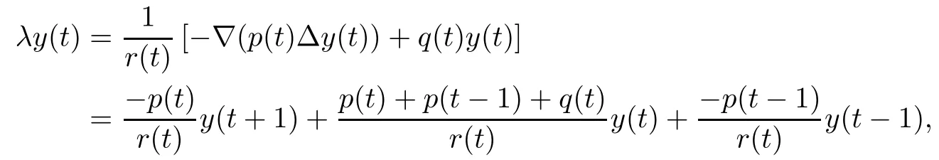
For the discrete case, there are also several interesting eigenvalue results on the problems with eigenparameter-dependent boundary conditions; see, [14, 24–26, 29, 30, 37, 38, 48], and the references therein. In particular, Harmsen and Li [29] considered the discrete right definite eigenvalue problem
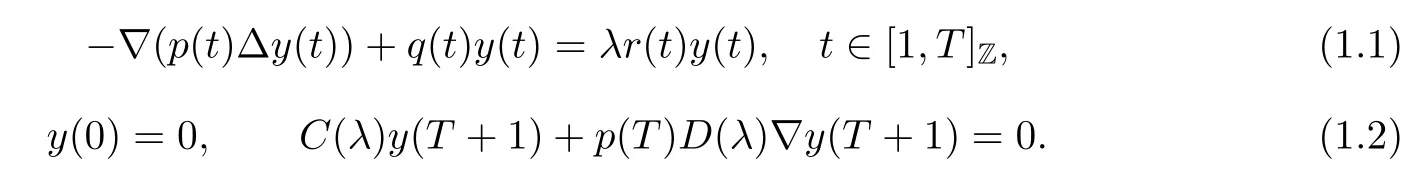
Here, ?y(t) = y(t)?y(t ?1), ?y(t) = y(t+1)?y(t), [1,T]Z= {1,2,···,T}, λ is a spectral parameter, C(λ) = c0+c1λ+c2λ2, and D(λ) = d0+d1λ+d2λ2. It is obtained that all the eigenvalues of the problem (1.1), (1.2) are real and simple, and the number of the eigenvalues is at most T +2. The conditions they used are as follows:
(H1) p(t)>0 for t ∈[0,T]Z; r(t)>0 on [1,T]Z;
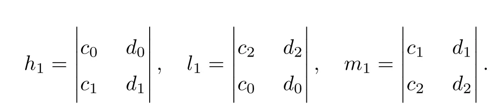
(H2) c2≠=0,d2≠=0, and M1is a positive definite matrix, where

and
After this, under the same conditions, Gao et al. [25] also considered the spectra of the problem (1.1), (1.2) (actually, they considered the problem under a more general boundary condition, that is, b0y(0)=d0?y(0)). Under the conditions (H1) and (H2), they obtained the exact number of the eigenvalues of the problem (1.1), (1.2) as coefficients ciand divary. That is, the problem (1.1), (1.2) have T +1 or T +2 eigenvalues at different cases. Furthermore,they obtained interlacing properties of eigenvalues and oscillation properties of corresponding eigenfunctions.
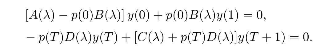
However, in [25, 29], the problem has only one squared eigenparameter-dependent boundary condition. Naturally, the question is: Could we also obtain the spectra of the eigenvalue problems with two squared eigenparameter-dependent boundary conditions? In fact,the eigenvalue problems with squared eigenparameter-dependent boundary conditions could be deduced in different fields [8, 32–34]. Therefore, inspired by the above results, we try to discuss the spectra of (1.1) with two squared eigenparameter-dependent boundary conditions as follows and try to give more rich results on the spectrum

Here, A(λ) = a0+a1λ+a2λ2, and B(λ) = b0+b1λ+b2λ2. As both boundary conditions here are with quadratic spectral parameters, to obtain the existence of real eigenvalues of the eigenvalue problems (1.1), (1.3) will be more difficult. To get that, besides (H1) and (H2), a new condition on A(λ) and B(λ) is introduced as follows:

and

Under the conditions (H1)–(H3), by constructing the appropriate Hilbert space, we will prove that the corresponding operator of the problem is self-adjoint; see Section 5. Furthermore,more basic properties including the orthogonality of the eigenfunctions and the expansion theorem will be obtained in this section. It is obvious that our results in Section 5 generalized the results of [29]. Meanwhile, from Section 2 to Section 4, the existence, the simplicity,the interlacing property and the exact number of eigenvalues will be obtained by constructing some new Lagrange-type identities, and two fundamental functions; see Section 2 and Section 3. In Section 4, by constructing a new oscillation theorem for solutions of initial problems, the oscillation properties of the eigenfunctions were obtained. Combining Section 3 with Section 4,we obtain some results those are different from the classical eigenvalue problem: (a)The“first”eigenvalue (whose eigenfunctions have the constant sign) may not exist; see, for instance, Theorem 3.3–Theorem 3.5. (b) The “first” eigenvalue may be not only one, see Theorem 3.4 as k0= 0. Moreover, in Section 4, some exceptional cases were noticed, which means although the assumption (H2) or/and (H3) does/do not hold, we could also obtain real eigenvalues of eigenvalue problems (Remark 4.7). In particular, in some exceptional cases, our results will reduce to the results of [24, 25]; and the classical eigenvalue results in [7, 22, 31, 35]. In Section 6, we convert our problem to a matrix problem, which could be a computation scheme for us to compute eigenvalues and eigenfunctions of specific eigenvalue problems by using the mathematical software like Matlab. Meanwhile, as applications of this computation scheme,we compute eigenvalues and eigenfunctions of some specific examples, and these results could be used to illustrate our main theoretic results. Here, at last, it should be mentioned that the interlacing results and the oscillation results for the classical discrete Sturm-Liouville problems could be found in [13, 19, 22, 27, 28, 39, 41, 43–45], and references therein.
2 Preliminaries
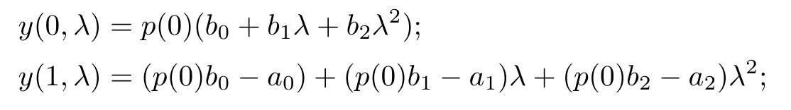
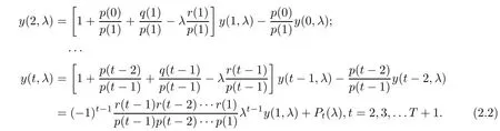
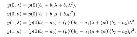
At first, let us construct a type of solution, y(t,λ), satisfying (1.1), and the first boundary condition in (1.3). That is, the solution y(t,λ) satisfies the initial conditions:

and the following generalized Sturm’s sequences:
Now, as a corollary of [6, Lemma 4.6–4.7], we obtain the following lemma for C(λ) and D(λ).
Lemma 2.1Suppose that (H2) holds. Then, both C(λ) and D(λ) have two distinct real roots. Meanwhile, these four roots are different.
Meanwhile, similar to the proof of [6, Lemma 4.6–4.7], we also obtain the properties for A(λ), B(λ).
Lemma 2.2Suppose that (H3) holds. Then, both A(λ) and B(λ) have two distinct real roots. Meanwhile, these four roots are different.
Lemma 2.3Suppose that (H1) and (H3) hold. If y(t,λ) is a solution of the initial value problem (1.1)λ, (2.1) and y(t,μ) is a solution of (1.1)μ, (2.1), then for t ∈[1,T]Z,

ProofAt first, (1.1)λand (1.1)μare rewritten, respectively, as follows:
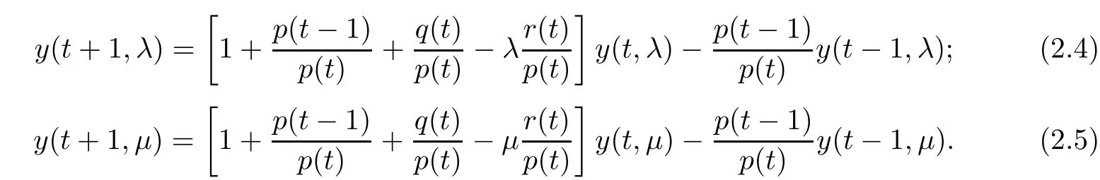
Multiplying (2.4) by y(t,μ) and (2.5) by y(t,λ) and then subtracting, we have
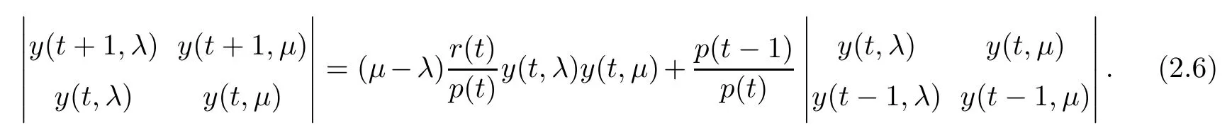
By (2.2), we know that
Then, (2.6) implies that
Now, by induction over t, (2.3) holds.
In Lemma 2.3, if we divide (2.3) by μ?λ and make μ→λ for fixed λ, then the following Langrange-type identity holds.
Corollary 2.4Suppose that (H1) and (H3) hold. If y(t,λ) is a solution of the initial value problem (1.1), (2.1), then for t ∈[1,T]Z, we have
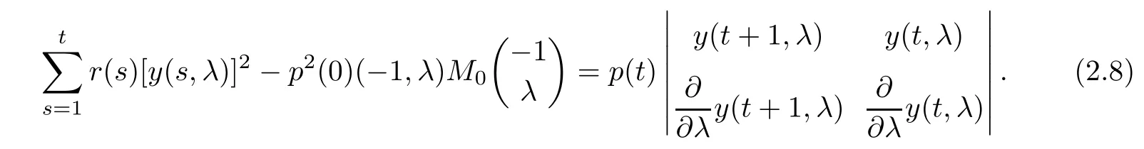
Furthermore, for complex λ, we obtain the following Langrange-type identity.
Corollary 2.5For t ∈[1,T]Zand complex λ, we have

ProofPut μ=in (2.3), and
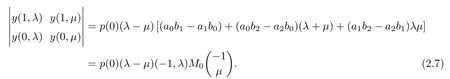
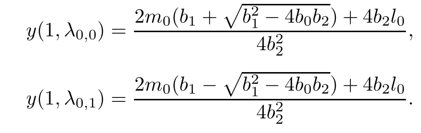
Lemma 2.6Suppose that (H1) and (H3) hold. Then, y(0,λ) = 0 has two real and simple roots λ0,0and λ0,1, and y(t,λ) = 0 has t+1 real and simple roots λt,s, s = 0,1,··· ,t,t=1,2,··· ,T +1.
ProofFirstly, by Lemma 2.2, both p(0)B(λ) and p(0)B(λ)?A(λ) have two distinct real roots and these four roots are different. Combining this with the expression of y(0,λ) and y(1,λ) in (2.2), we know that the result hold for t=0 and t=1.
Secondly, let t ∈[2,T + 1]Zand suppose on the contrary that λ is a complex zero of y(t,λ) = 0. Then, y(t,λ) = 0, y(t,) = 0. Combining this with Corollary 2.5, we know that the right of (2.9) equals zero. However, the left side of (2.9) are always positive by (H1) and(H3). Therefore, the zeros of y(t,λ) are all real. On the other hand, if y(t,λ) has a multiple zero, thenBy Corollary 2.4 and the assumptions(H1) and (H2), we also obtain a contradiction. Therefore, all the zeros of y(t,λ) are simple.
Finally, because y(t,λ) is a polynomial of λ with degree t+1 for t=1,2,··· ,T +1, then y(t,λ) have t+1 real and simple zeros.
As a consequence, similar to the eigenvalue results of [25], we obtain the eigenvalue results of the “Right Hand Dirichlet Problem(RDP)”, that is, (1.1) with the first boundary condition in (1.3)and y(T +1)=0, and the “Right Hand Neumann Problem(RNP)”, that is,(1.1) with the first boundary condition in (1.3) and ?y(T +1)=0.
Corollary 2.7Suppose that(H1)and(H2)hold. Then,both RDP and RNP have exactly T +2 real and simple eigenvalues,and, k =0,1,2,··· ,T +1, respectively. Meanwhile,these eigenvalues satisfy

Lemma 2.8Suppose that (H1) and (H3)hold. Then, two consecutive polynomials y(t ?1,λ), y(t,λ) have no common zeros. Furthermore, if λ = λ0is a root of y(t,λ), then y(t ?1,λ0)y(t+1,λ0)<0.
ProofFrom Lemma 2.2, we know that y(0,λ) and y(1,λ) do not have common zero.Then, for t ∈[2,T +1]Z, if there exists λ = λ0such that y(t ?1,λ0) = y(t,λ0) = 0. Then,by equation (1.1), we obtain y(t ?2,λ0) = 0. Furthermore, we obtain y(t ?3,λ0) = ··· =y(1,λ0)=y(0,λ0)=0. However, this contradicts the fact that y(0,λ) and y(1,λ) do not have common zero. Therefore, the first part of this lemma holds.
Next, if y(t,λ0) = 0, then by the first part, y(t ?1,λ0)0. Furthermore, by equation(1.1),

This completes the assertion.
3 Interlacing Properties of Eigenvalues
In this section, we try to look for eigenvalues of (1.1), (1.3) and obtain the interlacing property of eigenvalues of (1.1), (1.3).
Lemma 3.1Suppose that (H1), (H2), and (H3) hold. Then, the eigenvalues of (1.1),(1.3) are real and simple. Furthermore, all the eigenfunctions of (1.1), (1.3) are real.
ProofLet y(t,λ) be a solution of the initial problem (1.1), (2.1). Then, the eigenvalues of (1.1), (1.3) are the roots of

Firstly, let us prove that the eigenvalues of (1.1), (1.3) are real. Suppose on the contrary that (1.1), (1.3) has a nonreal eigenvalue λ?and the corresponding eigenfunction is y(t,λ?).
By Lemma 2.3 with λ=λ?, μ=, and t=T, we know that
The number and/or pattern of three often appears in fairy tales to provide rhythm and suspense92. The pattern adds drama and suspense while making the story easy to remember and follow. The third event often signals a change and/or ending for the listener/reader. A third time also disallows93 coincidence such as two repetitive events would suggest.Return to place in story.
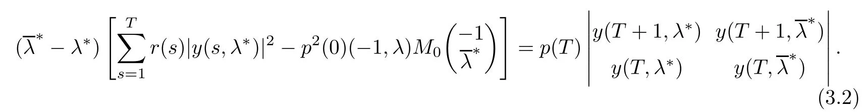
Combining this with the fact that λ?andare the roots of (3.1), it is obtained that the right side of (3.2) equals
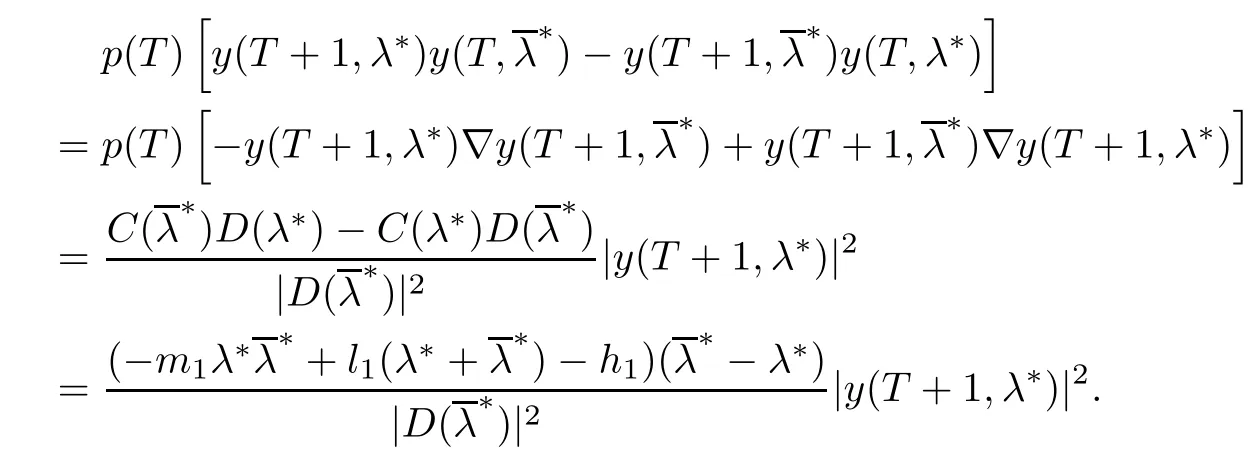
Therefore, (3.2) becomes
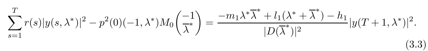
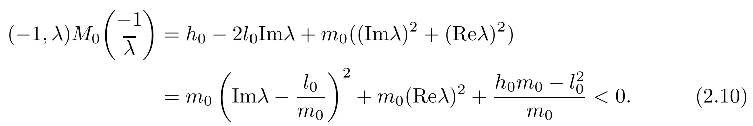
Furthermore, as
then, the right side of (3.3) is negative by (H1) and (H2). On the other hand, by (H1) and(H3), the left side of (3.3) is positive. A contradiction. Therefore, all the eigenvalues of (1.1),(1.3) are real.
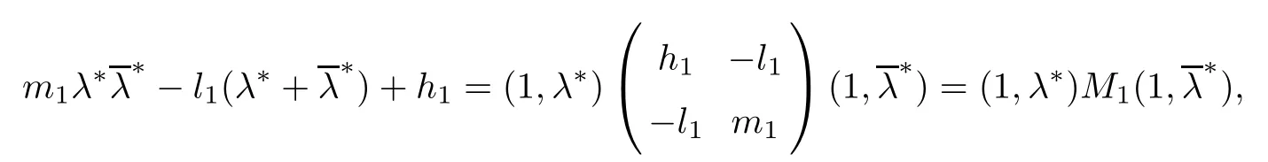
Secondly, let us show that all the roots of (3.2) are simple. Suppose on the contrary that(3.2) has a multiple zero, then

and
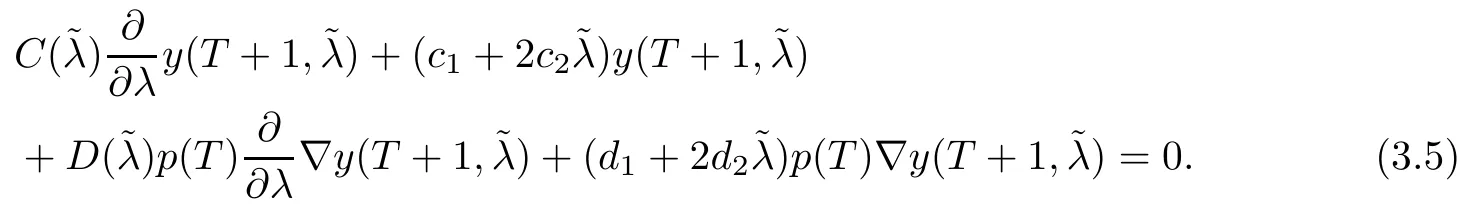
From Lemma 2.4 with t=T, we know that
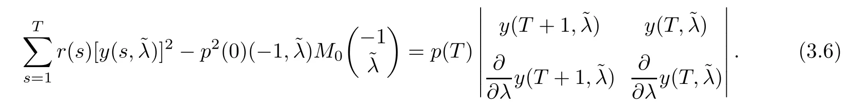
Furthermore, by Lemma 2.2,C(λ) and D(λ) do not have the same zero-point. So, without loss of generality, let. Then, by (3.4), (3.5), and (3.6), we have

By (H1) and (H3), we know that the left side of (3.7) is positive. However, by (H2), the right side of (3.7) is negative. A contradiction. Therefore, all the roots of (3.1) are simple.
Finally, because all the roots of (3.1) are real, which implies that all the eigenvalues of(1.1), (1.3) are real. Combining this with (2.2), then, all the eigenfunctions of (1.1), (1.3) are real.
To obtain it, we shall define two fundamental functions f(λ) and g(λ) as follows. Letbe defined as
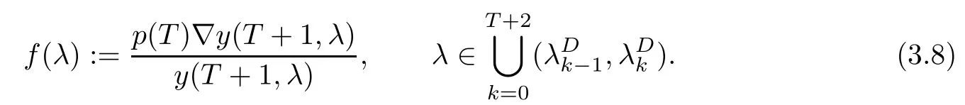

where ν1and ν2are two roots of D(λ) = 0. By Lemma 2.1, ν1and ν2are two real numbers with ν1≠ν2. Without loss of generality, we always assume that ν1< ν2in the rest of our article.
Now,finding the roots of f(λ)=g(λ)is equivalent to finding the eigenvalues of (1.1),(1.3).
At first, let us discuss some properties of f(λ) and g(λ) as follows.
Lemma 3.2Suppose that (H1) and (H3) hold. Then, f(λ) has following properties:
(i) The graph of f(λ)has T+3 branches,k =0,1,··· ,T+2. For each k =0,1,··· ,T+1,intersects λ-axis at λ=;
(ii) f(λ) is (strictly) decreasing as λ varies fromto, for k =0,1,··· ,T +2;
(iii) For k = 0,1,··· ,T, f(λ) →+∞as λ ↓and f(λ) →?∞as λ ↑. Meanwhile,f(λ)→p(T) as λ →±∞.
ProofAs y(T +1,λDk)=0 and ?y(T +1,)0, then, (i) holds.
(ii) From (3.8), we know that if λ ∈(), then f(λ) is well-defined and

Thus, (ii) holds.
(iii) For k = 0,1,··· ,T, we know that y(T +1,)= 0, but y(T,)0. Thus, by the definition of f(λ) in (3.8) and (ii), we see that f(λ) →+∞as λ ↓and f(λ) →?∞as λ ↑. Furthermore, as ?y(T +1,λ) and y(T +1,λ) are two polynomials of degree precisely T +2 of λ and the coefficients of the highest term are both (?1)Tp(T),we obtain f(λ)→p(T)as λ →±∞.
Lemma 3.3Suppose that (H1) and (H3) hold. Then, g(λ) has following properties:
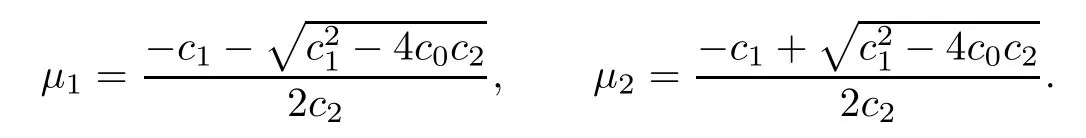
(i) g(λ) has two different real zeros μ1and μ2with
Meanwhile, the graph of g(λ) has three branches Dk, k = 0,1,2 with two vertical asymptotes λ=ν1and λ=ν2.
(ii) g(λ) is (strictly) increasing for λ ∈(?∞,ν1) or λ ∈(ν1,ν2) or λ ∈(ν2,∞).
(iii)

ProofBy Lemma 2.1, it is easy to see that the first assertion (i) holds. Meanwhile, if(ii) holds, it is also easy to see that the third assertion (iii) holds. Now, we only need to prove that assertion (ii) holds. In fact, for λ ∈(?∞,ν1)∪(ν1,ν2)∪(ν2,∞), we have
Then, by (H2), we know that h1> 0, h1m1?> 0, and m1> 0. Therefore, g′(λ) > 0 for λ ∈(?∞,ν1), λ ∈(ν1,ν2) or λ ∈(ν2,+∞). This implies that g(λ) is (strictly) increasing on each of its branches.
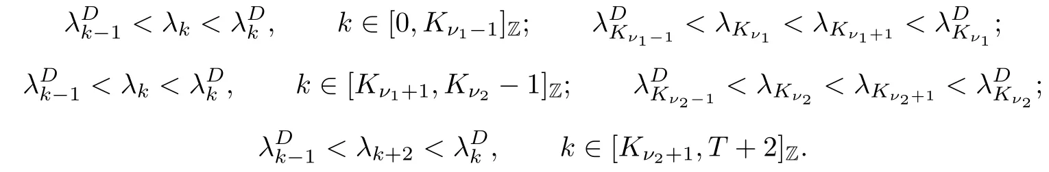
Suppose that the line λ = ν1intersects the Kν1-th branch and λ = ν2intersects the Kν2-th branch of f or their right hand asymptotes, that is, we select two nonnegative integers Kν1:0 ≤Kν1≤T +1 and Kν2:0 ≤Kν2≤T +1 such that

Define two integers Lμ1and Lμ2with 0 ≤Lμ1,Lμ2≤T +1 such that

Without loss of generality,suppose thatμ1<μ2and ν1<ν2. Then,Kν1≤Kν2and Lμ1≤Lμ2.
Furthermore, the properties of g(λ) implies that Lμ1≤Kν1≤Lμ2≤Kν2for ?> 0 and Kν1≤Lμ1≤Kν2≤Lμ2for<0.
Now, we discuss the case that>p(T). According to relations of Kν1and Kν2, we can obtain the following three existence, interlacing results as follows. We also obtain the fact that(1.1), (1.3) have T +4 eigenvalues in this case.
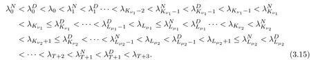
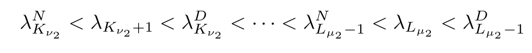
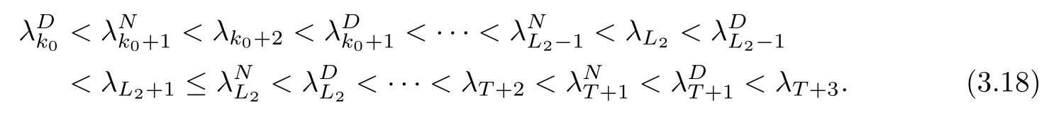
Theorem 3.4Suppose that (H1)–(H3) hold. If> p(T) and Kν1< Kν2, then the problem (1.1), (1.3) has T +4 real eigenvalues. More precisely, these eigenvalues satisfy the following interlacing inequalities:
(a) If Kν2≤T +1, then
Here,λ0=unless ν1=,λLμ1=unlessμ1=,λKν2+1=unless ν2=,and λL2+1=unless μ2=
(b) If Kν2=T +2,
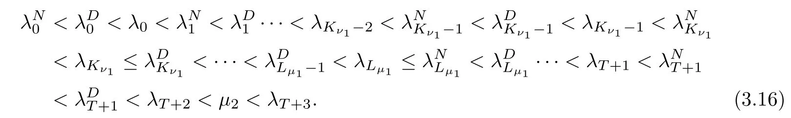
Here, λ0=unless ν1=, and λLμ1=unless μ1=.
Proof(a) Firstly, as> p(T), then, C0does not intersect the branch. Furthermore, from the assumption Kν1> 0, the branchwill intersect the upper parts of the branches of f(λ) fromto. Therefore,by the monotonicity of f(λ) and g(λ), we obtain the following interlacing inequality:

Secondly,let us consider the second branchof g(λ). If ν1<λKν1,then by the monotonicity of f(λ) and g(λ), D1will intersect branches of f(λ) fromto. More precisely,as Kν1≤Lμ1≤Kν2, we know that if μ1<, thenwill intersect the lower parts of branches of f(λ) fromto. Meanwhile,will intersect the upper parts of branches of f(λ) fromto. Therefore, by the monotonicity of f(λ) and g(λ), we obtain

and

Now, we consider the exceptional cases μ1=and ν1=. In fact, by Lemma 2.1,C(μ1) = 0 and D(μ1)0. Therefore, by the second boundary condition in (1.3), if μ1=, then ?y(T +1,μ1) = 0. This implies that μ1=is an eigenvalue of (1.1), (1.3).Furthermore, λLμ1=. Similarly, we also obtain the fact thatis an eigenvalue of the eigenvalue problem if ν1=and λKν1=.
Thirdly, let us consider the last branchof g(λ). If ν2< λKν2, thenintersects the branches of f(λ) fromto. More precisely, because Kν2≤Lν2, we obtain the result that if μ2< λLμ2, thenintersects the upper parts of the branches of f(λ) fromto. Meanwhile,intersects the lower parts of the branches of f(λ)fromto.
Therefore, the rest eigenvalues satisfy
and

(b) We only need to consider the last two eigenvalues, because other T +2 eigenvalues could be obtained as part (a). In fact, if Kν2= T +2, then Lμ2= T +2 andTherefore, the discussion is slightly different from part (a). Actually, in this case,andboth intersect. However,is located at the left of λ = μ2and D2is located at the right of λ = μ2. Therefore, we obtain the last two eigenvalues of the problem which satisfy λT+2<μ2<λT+3. Thus, (3.16) holds.
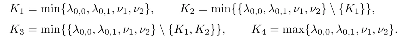
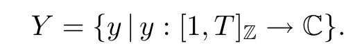
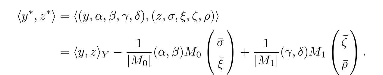
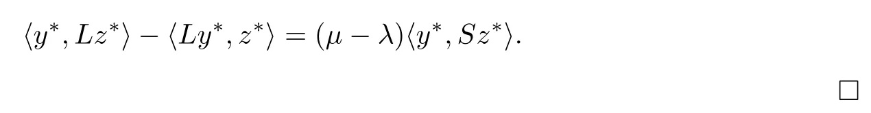
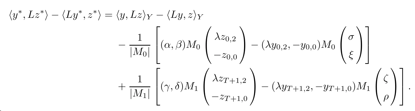
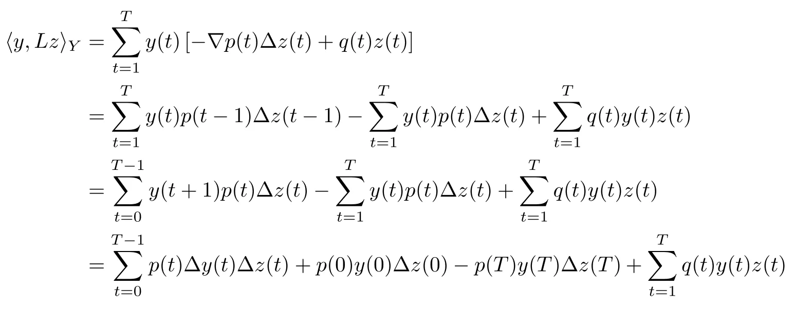
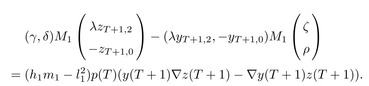
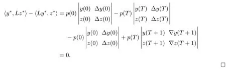
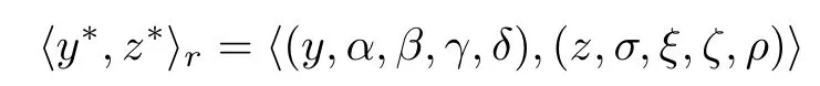
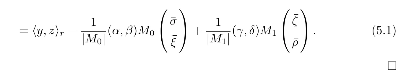
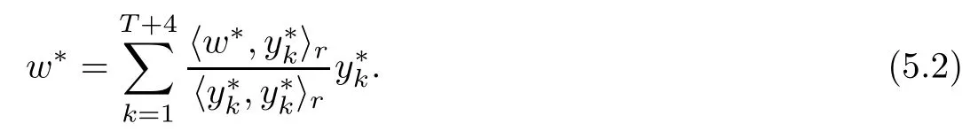
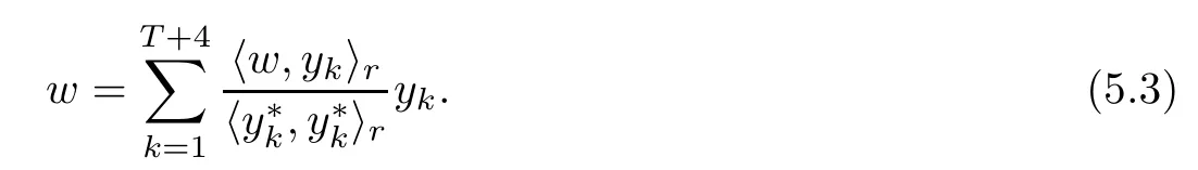
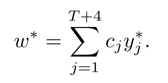
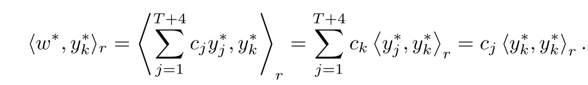
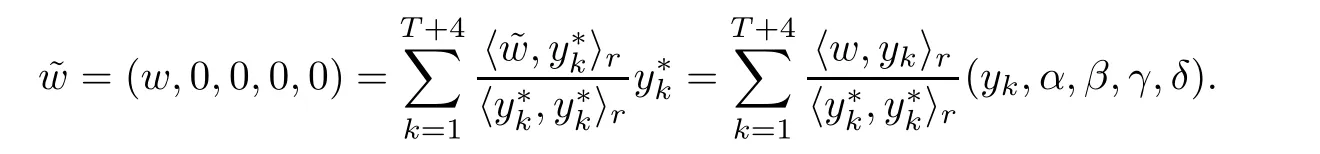
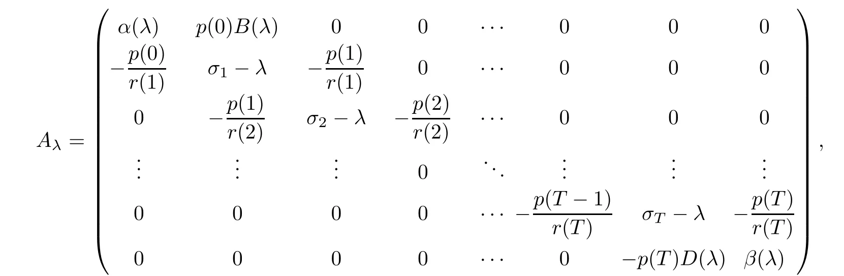
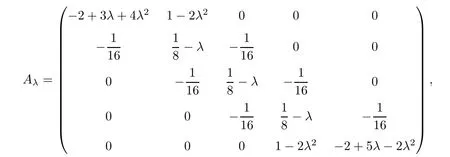
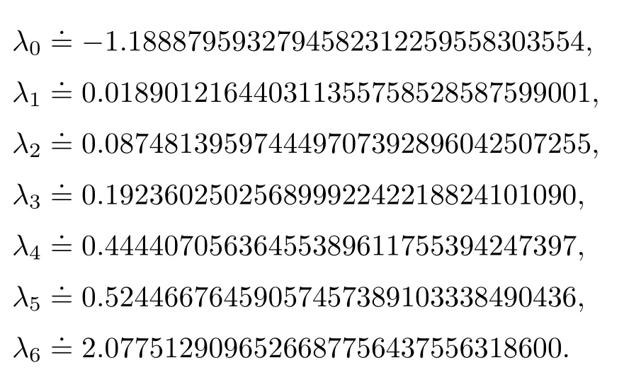
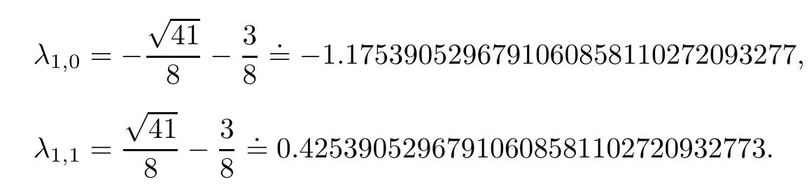
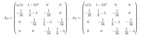
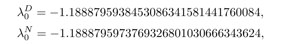
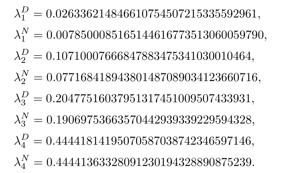
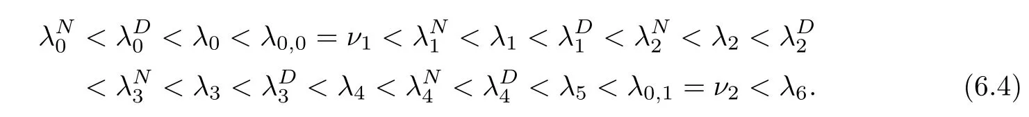
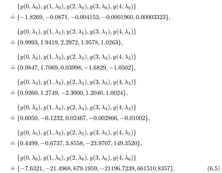
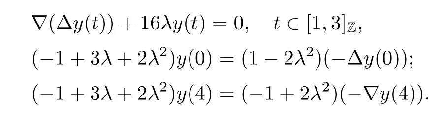
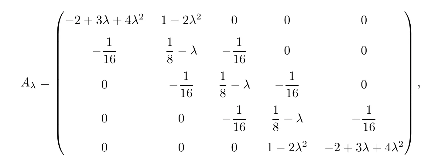
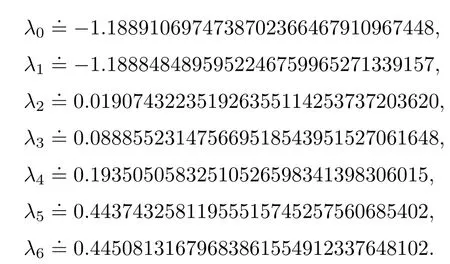
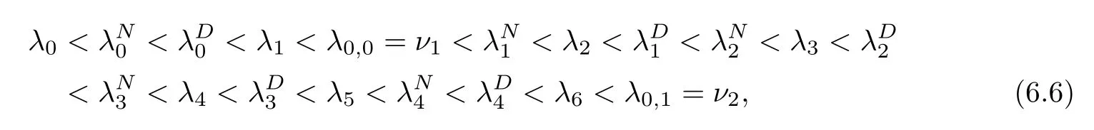
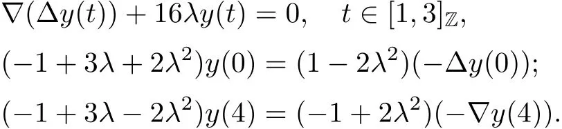
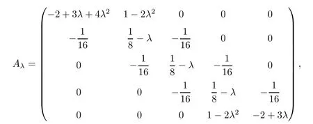
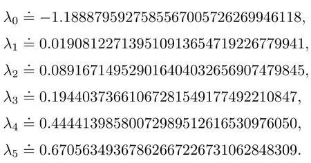
Theorem 3.5Suppose that (H1)–(H3) hold. If> p(T) and there exists k0∈[0,T +1]Zsuch that 0 ≤Kν1=Kν2=k0 and Meanwhile, the k0?1-th, k0-th, and k0+ 1-th eigenvalues satisfy the following interlacing inequalities: In particular, λk0 ProofAs in the proof of Theorem 3.4,because>p(T),the first branch,, of g(λ)does not intersect. Now, without loss of generality, we only consider the case that k0> 0,the case that k0=0 could be treated similarly. Firstly, by the monotonicity of f(λ) and g(λ),will intersect the upper parts of the branches of f(λ) fromto. Then, we have Therefore, (3.17) holds. Secondly, as Kν1= Kν2= k0, we know that< ν1< μ1< ν2≤. Obviously,(μ1,0) is the only intersection point ofand λ-axis. Therefore, by the monotonicity of g(λ),if μ1<, thenintersects the upper part of. Therefore, if μ1<, then combining this with (3.21), we obtain By the assumption, we know that ν1<μ1<ν2. Thus, iforν2with μ1<λk0, then. Therefore, (3.22) holds for both of these two cases. If μ1=, thenintersectsat (,0)and if μ1>, thenintersects the lower part of. Combining this with the second boundary condition in (1.3), thenis the k0-th eigenvalue of the eigenvalue problem (1.1), (1.3). Ifμ1>,thenintersects the lower part of Ck0. Therefore,ifμ1>,then combining this with (3.21), we have Finally, for the third branch D2of g(λ), it always intersects the lower parts of the branches fromtoand the lower parts of the branches fromto. Meanwhile,does not intersects the upper part of CLμ2all the times. Actually, it intersects the lower part ofwhen μ2 Similar to the proof of Theorem 3.5, we could also obtain the interlacing result for Kν1=Kν2= T +2. The only difference between this case and the case that Kν1= Kν2< T +2 is the last three eigenvalues. These three eigenvalues could not be separated byor.They have to be separated by μ1and μ2. The reason for this case is thatwill intersect the branches fromto.andonly intersect the branch. Therefore, we obtain the following interlacing properties for the eigenvalues. Theorem 3.6Suppose that (H1)-(H3) hold. If> p(T) and Kν1= Kν2= T +2,then (1.1), (1.3) has T +4 real eigenvalues. These eigenvalues satisfy Remark 3.7Similar discussions could be used to discuss the cases thatandFor the case that, the eigenvalues of the problems are not T +4, but T +3. Meanwhile, the interlacing properties also hold for these T +3 eigenvalues if we get rid of λT+3from (3.15), (3.16), (3.18), and (3.24). For the case that, it have to be divided into two cases:andbecause the location of the zero points of g(λ) are different. Other discussions are similar to those of Theorems 3.4–3.6. So, we omit them here. In this section, we try to obtain the oscillation properties of the eigenfunctions. First of all,let us discuss the oscillation properties for the initial problem (1.1), (2.1), which will play an important role in discussing the oscillation property of eigenfunctions of (1.1),(1.3). At first,let us discuss some properties for the generalized Sturm’s sequence (2.2), that is, the relationship of zeros of each polynomial y(t,λ) for t=0,1,··· ,T +1. Lemma 4.1Suppose that (H3) holds. Then, the roots of y(0,λ)=0 and y(1,λ)=0 are separated from each other. ProofBy Lemma 2.2,we know that both y(0,λ)and y(1,λ)have two distinct real roots. Let λ0,0,λ0,1be two roots of y(0,λ) asandThen Then, by assumption (H3), we obtain Therefore,y(1,λ0,0)y(1,λ0,1)<0. Combining this with Lemma 2.4,then y(1,λ0,0)and y(1,λ0,1)have opposite signs, which proves the result. Remark 4.2From Lemma 4.1, we know that the roots of y(0,λ)=0 and y(1,λ)=0 are separated from each other. However,if we try to discuss the relation of the roots of y(1,λ)=0 and y(2,λ)=0, then the relation of λ0,0, λ1,0and the signs of p(0)b2?a2, p(0)b2will play an important role. In fact,if(p(0)b2?a2)(p(0)b2)>0 and λ0,0>λ1,0,or(p(0)b2?a2)(p(0)b2)<0 and λ0,0< λ1,0, then the roots of y(1,λ) = 0 and y(2,λ) = 0 satisfy the following interlacing inequalities: Therefore, without loss of generality, in the rest of this article, let us suppose that (H4) (p(0)b2?a2)p(0)b2>0 and λ0,0>λ1,0. Lemma 4.3Suppose that (H1), (H3), and (H4) hold. Then, for t ∈[0,T]Z, the roots of y(t,λ)=0 and y(t+1,λ)=0 separate each other. ProofThis result will be proved by induction. Firstly, by Lemma 4.1 and Remark 4.2,the result holds for t=0 and t=1. Secondly, suppose that the roots of y(k ?1,λ) = 0 and y(k,λ) = 0 separate each other for t = k ?1. For details, the roots of y(k ?1,λ) = 0 and the roots of y(k,λ) = 0 satisfy the following interlacing inequalities: Furthermore, because y(k ?1,?∞)>0 and y(k ?1,λk?1,s)=0, for s=0,1,··· ,k ?1, it can be seen that Combining this with Lemma 2.8, we obtain Thus, combining this with the fact thatwe know that y(t,λ) has at least one root in each of the k+2 intervals(?∞,λk,0),(λk,0,λk,1),··· ,(λk,k?1,λk,k),(λk,k,+∞). On the other hand, as y(k+1,λ)is a polynomial of λ with degree k+2,it has at most k+2 zeros.Therefore, there is only one root of y(k+1,λ)=0 in each interval. Hence, by the method of mathematical induction, the result of Lemma 4.3 holds. Now, we consider the oscillation properties of nontrivial solutions of the initial problem(1.1), (2.1). By assumption (H4), there exist four nonnegative constants K0,0, K0,1, K1,0, and K1,1with 0 ≤K1,0≤K0,0≤K1,1≤K0,1≤T +1 such that and Lemma 4.4Suppose that (H1), (H3), and (H4) hold. Then (a) for each k ∈[0,K0,0?1]Z, if λ ∈(] or λ ∈[,λ0,0) , then all solutions of (1.1), (2.1) change their signs exactly k times in [0,T +1]Z; (b) for each k ∈[K0,0,K0,1?1]Z,if λ ∈(]or λ ∈[λ0,0,]or λ ∈[,λ0,1),then all solutions of (1.1), (2.1) change their signs exactly k ?1 times in [0,T +1]Z; (c) for each k ∈[K0,1,T +1]Z, if λ ∈(,] or λ ∈[λ0,1,], then all solutions of(1.1), (2.1) change their signs exactly k ?2 times in [0,T +1]Z. ProofIt is necessary to prove the sign-changing times of the following Sturm’s sequence At first, we consider sign-changing time of the sequence By Lemma 4.4 and the similar proof of Lemma 2.3 in [24, 26], we obtain the fact that Now, let us prove (a) firstly. In fact, by (H4), we know that λ0,0> λ1,0and= +∞. Therefore, if λ < λ1,0, then sequence (4.2) and sequence (4.3) has the sign-changing times. Combining this with (P1), we know that (4.2) changes its sign exactly k times for λ < λ1,0. Meanwhile, if λ ∈(λ1,0,λ0,0), then by (H4), y(0,λ) > 0 and y(1,λ) < 0. Therefore,the sign-changing time of (4.2) is 1 time more than (4.3). If λ = λ1,0, then y(0,λ) > 0,y(1,λ)=0. By Lemma 2.8,y(2,λ)<0. Therefore,we obtain the same result as λ ∈(λ1,0,λ0,0).Therefore, the assertion (a) holds. Secondly, let us consider the assertion (b). In fact, if λ ∈[λ0,0,λ1,1), then by Lemma 2.8,y(0,λ)≤0 and y(1,λ)<0. Therefore,the sign-changing times of (4.2)and(4.3)are the same.If λ ∈(λ1,1,λ0,1), then y(1,λ)> 0 and y(0,λ)<0. Therefore, the sign-changing time of (4.2)is 1 time more than(4.3). If λ=λ1,1, then y(0,λ)<0,y(1,λ)=0. By Lemma 2.8,y(2,λ)<0.Therefore, we obtain the same result as λ ∈(λ1,1,λ0,1). Therefore, (b) holds. Thirdly, if λ ∈[λ0,1,+∞), then y(1,λ) > 0 and y(0,λ) > 0. Therefore, the sign-changing times of (4.2) and (4.3) are the same, which implies that (c) holds. For the sake of convenience, let Then, K1≤K2≤K3≤K4, K1=min{λ0,0,ν1} and K4=max{λ0,1,ν2}. Theorem 4.5Suppose that(H1)–(H4)hold and>p(T). If K1=λ0,0or K1=ν1≥, then (a) if λk≤K1, then the corresponding eigenfunction yk(t) changes its sign exactly k+1 times on [0,T +1]Z; (b) if K1<λk≤K2, then the corresponding eigenfunction yk(t) changes its sign exactly k times on [0,T +1]Z; (c) if K2< λk≤K3, then the corresponding eigenfunction yk(t) changes its sign exactly k ?1 times on [0,T +1]Z; (d) if K3<λk≤K4, then the corresponding eigenfunction yk(t) changes its sign exactly k ?2 times on [0,T +1]Z; (e) if λk> K4, then the corresponding eigenfunction yk(t) changes its sign exactly k ?3 times on [0,T +1]Z. ProofWithout loss of generality, suppose that λ0,0<ν1<λ0,1<ν2. Other cases could be treated similarly. In this case, K0,0≤Kν1≤K0,1≤Kν2. Firstly, by Lemma 4.4, λ0,0>. Meanwhile, by Theorems 3.4–3.6,< λk If ν1< λk< λ0,1, then by Theorems 3.4–3.6, we know that< λk Similarly, if λ0,1≤λk< ν2, then by Theorems 3.4–3.6,< λk Finally, if λk>ν2, then by Theorems 3.4–3.6, we obtain<λk Remark 4.6From Theorem 4.5, we know that the sign-changing time of eigenfunctions mainly dependents on the relations of Ki. Furthermore, we could find that if no λkis in(Ki?1,Ki] for some i = 0,1,2,3,4,5 (here, K?1= ?∞and K5= +∞), then all of eigenfunctions do not change its time k ?i+2. Theorem 4.7Suppose that (H1)–(H4) hold and>p(T). If K1=ν1<, then (a) if λk≤K1, then the corresponding eigenfunction yk(t)changes its sign exactly k times on [0,T +1]Z; (b) if K1<λk≤K2, then the corresponding eigenfunction yk(t) changes its sign exactly k ?1 times on [0,T +1]Z; (c) if K2< λk≤K3, then the corresponding eigenfunction yk(t) changes its sign exactly k ?2 times on [0,T +1]Z; (d) if K3<λk≤K4, then the corresponding eigenfunction yk(t) changes its sign exactly k ?3 times on [0,T +1]Z; (e) if λk> K4, then the corresponding eigenfunction yk(t) changes its sign exactly k ?4 times on [0,T +1]Z. ProofThe main reason that causes the differences of Theorem 4.5 and Theorem 4.7 is the interlacing properties of eigenvalues. In fact, from Theorem 3.4 and Theorem 3.5, if K1=ν1<, then Therefore, similar to the proof of Theorem 4.5, the results of Theorem 4.7 hold. Remark 4.8Similar to the discussion of Remark 4.6, in some cases, the sign-changing time will not always strictly obey the rule: k, k ?1,k ?2,k ?3,k ?4. Remark 4.9In this article, we always suppose that (H2) and (H3) hold. Now, let us focus on some exceptional cases. Case IIf a2= b2= c2= d2= 0, then l0= m0= 0 = l1= m1and M0is not a seminegative definite matrix, and M1is not a semi-positive definite matrix. Therefore, (H2) and(H3) do not hold. However, the problem we considered here reduces to the problem in [24].Furthermore, in this case, h0=a0b1?a1b0and h1=c0d1?c1d0. Then, if h0<0 and h1>0,our results will reduces to the results of [24]. Case IIIf a2=a1=b2=b1=0, but (H3) holds. Then l0=m0=h0=0, which imples that M0is a semi-negative matrix and M1is a positive definite matrix. Then, our results will reduce to the results of [25, 29]. Case IIIIf p(0)b2?a2= 0, then y(1,λ) = (p(0)b1?a1)λ+(p(0)b0?a0). Therefore,y(t,λ)is a polynomial of λ with degree t. Therefore,if M0is negative definite, then y(T+1,λ)has exactly T +1 real eigenvalues. Furthermore, similar to the discussion of Theorems 3.4–3.6,if (H3) holds, then the eigenvalue problem (1.1), (1.3) has exactly T +3 eigenvalues. However,the sign-changing time of the corresponding eigenfunction will have some changes. In fact, if b20, then the results of Lemma 4.4 will hold like: (a) if λ ∈(?∞,λ0,0), then the signchanging time of nontrivial solution y(t,λ) of (1.1), (2.1)is k times; (b) if λ ∈(λ0,0,λ0,1), then the sign-changing time is k ?1 times; (c) if λ ∈(λ0,1,+∞), then the sign-changing time is k times. Because the results (c) arise, therefore, the sign-changing time of the eigenfunction also has a big change. That is the sign-changing time does not strictly obey the rule: k+1,k, k ?1,k ?2, k ?3. More precisely, the sign-changing time may obey the rules: k+1, k, k ?1, k ?1,k ?2 or k+1,k, k ?1, k ?2, k ?2,and so on. Meanwhile,the similar discussion will also hold for the cases: b2=0, but p(0)?a20 and p(0)b2?a2=b2=0 (in this case, |M0|=0). Case IVIf (H2) holds, but (H3) does not hold. Then, we may discuss some exceptional cases as: (i) c2= 0, but d20; (ii) d2= 0, but c20; (iii) c2= d2= 0 (in this case,|M1|=0). Similar to the discussion of[25]and Case III,we could also obtain the exact number of eigenvalues and the sign-changing time of the corresponding eigenfunctions. In particular,the sign-changing time of the eigenfunction also may not strictly obey the rule: k+1,k, k ?1,k ?2, and k ?3. At last, we try to consider some properties of the corresponding operator to the eigenvalue problem and try to obtain the orthogonality of the eigenfunction,and then obtain the expansion theorem. To obtain it, we always suppose that (H1), (H2), and (H3) hold in this section. Let Then, Y is a Hilbert space under the inner product Furthermore, consider the space H :=Y ⊕C4with the inner product given by Let y0,0= a0y(0)+b0p(0)?y(0), y0,1= a1y(0)+b1p(0)?y(0), y0,2= a2y(0)+b2p(0)?y(0).yT+1,0= c0y(T +1)+d0p(T)?y(T +1), yT+1,1= c1y(T +1)+d1p(T)?y(T +1), yT+1,2=c2y(T+1)+d2p(T)?y(T+1). Then,the boundary conditions(1.3)is equivalent to the following form: where Ly = ??(p(t)?y(t)) + q(t)y(t) and D(L) = {(y,α,β,γ,δ)|y ∈Y, y0,2= α, y0,1+λy0,2= β, yT+1,2= γ, yT+1,1+ λyT+1,2= δ}. Define another operator S : Y →Y by That is, if (λ,y) is an eigenpair of the problem (1.1), (1.3), then (λ,) is an eigenpair of L.Conversely, if (λ,) is an eigenpair of L, then (λ,y) is an eigenpair of the problem (1.1), (1.3). According to Lemma 3.1, all of the eigenpairs (λ,yk(t,λ)) are real. Now, let us consider the orthogonality of the eigenfunctions. Lemma 5.1Suppose that (λ,y?) and (μ,z?) are eigenpairs of L, whereand∈D(L).Then, ProofLet y?=(y,α,β,γ,δ)∈D(L), z?=(z,σ,ξ,ζ,ρ)∈D(L). Then, Similarly, Therefore, Lemma 5.2L is a self-adjoint operator in H. ProofAcoording to [6, Definition 7.5], it suffices to show that 〈y?,Lz?〉= 〈Ly?,z?〉for y?= (y,α,β,γ,δ) ∈D(L), z?= (z,σ,ξ,ζ,ρ) ∈D(L). Then from the inner product in H, we obtain and Therefore, On the other hand, and Furthermore, and Therefore, To obtain the orthogonal property of the eigenfunctions, we have to define another inner product (with respect to the weight r(t)) on H. At first, define the weighted inner product on Y byThen, the weighted inner product on H is defined as Theorem 5.3(Orthogonality Theorem) Suppose that (H1)–(H3) hold. Then, linear independent eigenfunctions of L are orthogonal under the weighted inner product defined as(5.1). ProofLet (λ,y?) and (μ,z?) be eigenpairs of L. Then, by Lemma 5.1 and Lemma 5.2, Now, let us consider the expansion theorem. Because (H1), (H2), and (H3) hold, we know that the space H is a T+4-dimension space. Furthermore,by Theorems 3.4–3.6,the eigenvalue problem has T +4 real and simple eigenvalues λk, and T +4 linear dependent and orthogonal eigenfunctions. Then, by Lemma 5.2, we will have the following expansion theorem. Theorem 5.4(Expansion Theorem) Suppose that (H1)–(H3) hold. Let (λk,) be an eigenpair of the operator L with=(yk,α,γ,β,δ). Then, for each w?=(w,α,β,γ,δ)∈H, Furthermore, ProofLet w?= (w,α,β,γ,δ) ∈H. Now, we try to find constants cj, j = 1,··· ,T +4 such that By Theorem 5.3, we know that Therefore, (5.2) holds. Therefore, (5.3) holds. Remark 5.5Now, some exceptional cases should be noted as Remark 4.9. In those four exceptional cases, the work space H may be a T +3 or T +2-dimensional space. However,after some obvious changes on the inner product, the orthogonality of the eigenfunctions and the expansion theorem could be obtained similarly. So, we omit them here. We use matrix form of the problem (1.1), (1.3) to obtain eigenvalues and corresponding functions. At first, we can rewrite the equation (1.1) as follows: and the boundary condition (1.3) is Then, the matrix equation corresponds to (1.1), (1.3) is where yT=(y0,y1,··· ,yT+1) and Aλis defined by where α(λ)=A(λ)?p(0)B(λ), β(λ)=C(λ)+p(T)D(λ), It could be seen that the matrix form of (1.1), (1.3) could also be a computation scheme to compute eigenvalues and eigenfunctions of (1.1), (1.3). Now, as applications, we give three specific examples in three cases:and Example 6.1Consider the following discrete Sturm-Liouville problem In this example, the corresponding matrix Aλis as follows: where h0=?3<0,m0=?6<0,|M0|=18>0,and h1=5>0,m1=10>0,|M1|=14>0. the roots of P(λ) are Moreover, and Obviously, λ0,0>λ1,0, λ0,1>λ1,1, and ν1=λ0,0, ν2=λ0,1. Then, Meanwhile,let us compute eigenvalues of RDP,that is,(6.1)with the boundary condition(6.2)and y(4) = 0, and eigenvalues of RNP, that is, (6.1) with the boundary condition (6.2) and?y(4)=0. Define two matrices as follows: Here, α(λ) = ?2+3λ+4λ2. Then, the RDP is equivalent to the matrix equation ADy = 0 and the RNP is equivalent to the matrix equation ANy = 0. Now, by computing the roots of the corresponding polynomials, we obtain the following real eigenvalues: Then, these eigenvalues satisfy the following interlacing results: As Kν1=1 and Kν2=T +2, the inequalities in (6.4) is the same to (3.16) in Theorem 3.4(b). Finally, we discuss the sign-changing times of the Sturm’s sequence: Let y(0,λ) = 1 ?2λ2and y(1,λ) = 2 ?3λ ?4λ2. By the recurrence relation y(t+1,λ) =(2 ?16λ)y(t,λ)?y(t ?1,λ) and Matlab 7.0, it is obtained that From(6.5),y0(t)changes its signs exactly 1 times in[1,4]Zand yi(t),i=1,2,3,4,5,change their signs exactly k ?1 times in [1,4]Z, y6(t) changes its signs exactly 3 times in [1,4]Z. Therefore,the oscillation properties of eigenfunctions of this problem is the same to the theoretic results in Theorem 4.6. Example 6.2Consider the following discrete Sturm-Liouville problem In this example, the corresponding matrix Aλis as follows: where h0=?3<0, m0=?6<0, |M0|=18>0, and h1=3>0,m1=6>0, |M1|=18>0. and the roots of P(λ) are Then, these eigenvalues satisfy the following interlacing results: where νi,,are the same to Example 6.1. We could use similar method of Example 6.1 to obtain oscillation properties for eigenfunction. So, we omit here. Example 6.3Consider the following discrete Sturm-Liouville problem In this example, the corresponding matrix Aλis as follows: where h0= ?3 < 0,m0= ?6 < 0,|M0| = 18 > 0 and h1= 3 > 0,m1= 6 > 0,|M1| = 2 > 0. the roots of P(λ) are Then, these eigenvalues satisfy the following interlacing results: where νi,,are the same to Example 6.1. We could use similar method of Example 6.1 to obtain oscillation properties for eigenfunction.


4 Oscillation Properties of Eigenfunctions
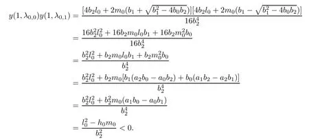


5 Self-adjoint Operator, Orthogonal Eigenfunction and Expansion Theorem


6 Numerical Results


 猜你喜歡
金山(2024年3期)2024-04-24 16:56:03美與時代·城市版(2022年6期)2022-05-30 07:28:40Journal of Donghua University(English Edition)(2022年2期)2022-05-09 06:48:08Journal of Donghua University(English Edition)(2022年2期)2022-05-09 06:48:04快樂作文(1.2年級)(2020年9期)2020-11-04 02:34:32小學(xué)生作文(低年級適用)(2020年3期)2020-03-28 03:38:52男生女生(金版)(2016年1期)2016-04-20 11:05:20鳳凰資訊報(2015年6期)2015-05-30 21:14:21讀者(2015年7期)2015-04-01 12:22:00文藝論壇(2015年23期)2015-03-04 07:57:15
猜你喜歡
金山(2024年3期)2024-04-24 16:56:03美與時代·城市版(2022年6期)2022-05-30 07:28:40Journal of Donghua University(English Edition)(2022年2期)2022-05-09 06:48:08Journal of Donghua University(English Edition)(2022年2期)2022-05-09 06:48:04快樂作文(1.2年級)(2020年9期)2020-11-04 02:34:32小學(xué)生作文(低年級適用)(2020年3期)2020-03-28 03:38:52男生女生(金版)(2016年1期)2016-04-20 11:05:20鳳凰資訊報(2015年6期)2015-05-30 21:14:21讀者(2015年7期)2015-04-01 12:22:00文藝論壇(2015年23期)2015-03-04 07:57:15
 Acta Mathematica Scientia(English Series)2020年3期