Combining spatial and economic criteria in tree-level harvest planning

Petteri Packalen,Timo Pukkala and Adrián Pascual

Abstract

Keywords: Spatial optimization, Tree selection, Cellular automata, Remote sensing,Airborne laser scanning

Background

Forest inventories employing Airborne Laser Scanning(ALS) data have become common in many countries(Nilsson et al. 2017). The ALS-based forest inventory methods (Hyypp? et al. 2008) are typically categorized into two groups: the area-based approach (ABA) (Means et al. 2000; N?sset 2002; Magnussen et al. 2013) and individual tree detection (ITD) (Hyypp? et al. 2001;Koch et al. 2006; L?hivaara et al. 2014). So far, most operational forest inventories employing ALS data have been implemented with the ABA (Maltamo et al. 2014).In ABA, stand attribute models are fitted with sample plots using metrics calculated from ALS data and then these models are used to predict stand attributes of the whole inventory area, typically using square grid cells(e.g. 16 m×16 m) as inventory units.

In ITD, the inventory unit is an individual tree. The first step is to detect and delineate the trees. Then ALS features, such as local maxima mimicking tree height,are extracted on a tree-by-tree basis and used to estimate tree-level attributes, such as tree height and diameter. Tree locations are also an intrinsic output of ITD.The disadvantage of ITD is that tree detection fails when tree crowns overlap, or if there are many small trees under the dominant tree layer (Falkowski et al. 2008;Lindberg et al. 2010). Failures in tree detection and errors in the prediction of tree attributes make ITD more sensitive to bias than ABA at the aggregated (e.g. forest stand) level (Vauhkonen 2010). However, the advantage of ITD is that it produces a more detailed description of forest: tree level attributes, including tree locations.

Forest plans are typically composed of homogenous regions for which inventory data are available. Most commonly,this region or inventory unit is a forest stand.In the ALS era, stand-level data are usually derived from ABA predictions in grid cells. In spatial forest planning,the inventory unit has been a stand (?hman 2000),microstand (Pascual et al. 2019), hexagon (Packalen et al. 2011)or pixel/cell(Lu and Eriksson 2000).To date,the use of tree-level data in forest or harvest planning has received limited attention. For example, Martín-Fernández and García-Abril (2005) developed a tree-level optimization method following an approach based on close-to-nature forestry, and Bettinger and Tang (2015)maximized the tree-level species mingling value in order to intersperse tree species across a forest. Algorithms have also been proposed for tree cut selection using a distance-dependent growth model (e.g. Pukkala and Miina 1998). Vauhkonen and Pukkala (2016) selected trees based on their value growth rate, and Pukkala et al.(2015) optimized the tree selection rule in thinning treatments when the profitability of forest management is maximized. These studies accounted for the location of trees when deciding the order in which to cut the trees. However, the spatial distribution of harvested trees was not controlled in optimization although it may be of great importance from ecological and practical viewpoints (Heinonen et al. 2018). Wing et al. (2019) implemented a method for group-selection silviculture that accounts for spatial aggregation, and utilized manually corrected stem map data that was derived by ITD.

Controlling the spatial distribution of individual harvested trees or other harvest units, such as micro-stands or stands, is possible both in mathematical programming(?hman 2002) and in heuristic planning methods(Heinonen et al. 2007). Heuristic methods are more flexible and may be easier to use in large and complicated spatial problems (Bettinger et al. 2002; Heinonen et al.2018). Two lines of heuristics have been developed for spatial forest planning problems: global and local methods (also called centralized and decentralized methods) (Heinonen and Pukkala 2007; Pukkala et al.2014). Common examples of centralized heuristics are simulated annealing, tabu search and genetic algorithms(Bettinger et al. 2002). Of the two categories of heuristics, decentralized methods may be faster and more feasible when the number of calculation units is very large,which is often the case in tree-level planning (Heinonen and Pukkala 2007).

Examples of decentralized heuristics are cellular automata (CA) (Strange et al. 2001, 2002; Mathey et al.2007) and the spatial version of the reduced cost method(Hoganson and Rose 1984; Pukkala et al. 2008). The aim of decentralized heuristics is to maximize or minimize a local objective function, which in tree-level planning is a tree-level function. This function is modified with a part that takes into account the global objectives or constraints of the planning problem. In the reduced costs method, global objectives are dealt with the dual prices of global constraints, whereas the applications of CA employ a global priority function that is added to the local function.

Cellular automata, which were used in the current study, are self-organizing algorithms based on the assumption that the interaction between cells decreases rapidly with increasing distance (Von Neumann 1966;Strange et al. 2001; Wolfram 2002). Although the name of the method refers to (square-shaped) cells, the method can also be used with other types of calculation units. Each unit takes one of a limited number of states,which can be management schedules, land uses or, as in the current study, the cut vs. uncut status of an individual tree. The purpose of CA is to find the optimal status for each cell,by considering the variables of the cell itself and the local neighborhood of the cell. The cell states evolve in discrete time steps according to a set of rules.Spatial relationships can be included in CA and other heuristic methods in various ways, for instance by considering only spatially adjacent calculation units(similar vs. different prescription), by also including the neighbors of adjacent units (Kurttila et al. 2002)or using distance as the criterion of neighborhood(Heinonen et al. 2018).

The aim of the study is to present a tree selection method that removes economically mature trees from the stand while also considering the spatial distribution of the harvested trees. A user controls whether the pattern of harvested trees is clustered or dispersed. We present a solution as to how tree-level data can be used in the spatial formulation of the optimization model common in forest and harvesting planning. The proposed method was tested in Central Spain on a stone pine (Pinus pinea L.) forest area with two different spatial distributions of trees. For this purpose, we implemented a simple ITD inventory, although the focus is on the tree selection algorithm.

Study area and materials

The study area is the public forest MUP50 owned by the municipality of Portillo in the province of Valladolid(366658-371652 Easting, 4590001-4586476 Northing,711-862 m a.s.l.) located in Castilla y León (Central Spain). The study area of 1100 ha consists of pure stone pine stands at different stages of development. The area is part of the Northern Plateau (Calama et al. 2008)where the stone pine forests are managed using evenaged forestry with the aim of providing a constant flow of revenue (timber, firewood and nut production) and other ecosystem services, such as erosion control(Calama et al. 2011).

We selected two sub-areas in a 78-year old stone pine forest. These two areas differed in average tree size and the spatial distribution of the trees (Fig.1). In Area #1(106.4 ha), the spatial distribution of the trees was more or less regular, i.e., tree spacing was somewhat constant.In Area #2 (47.9 ha), the trees grow more in groups and stand density and tree spacing was variable.

Field sample plots

Systematic sampling was used to establish a network of 35 circular sample plots in the area and used to model the relationship between tree height and diameter.Sample plots were collected in 2010. The size of each plot was 706.86 m2, i.e. circular plots with a radius of 15 m. The sample plots contained a total of 344 trees. The locations of the plot centers were determined by a submeter precision GNSS equipment (Garmin International Inc., Missouri, USA). On each plot, all trees with a diameter at breast height (DBH) over 7.5 cm were callipered and their heights were measured using a Vertex IV hypsometer (Hagl?f, Sweden). In addition, the distance and heading with respect to the plot center were determined with the distance meter and a Vertex IV compass (Hagl?f, Sweden). All the measured trees were stone pines. A summary of tree- and plot-level attributes is provided in Table 1.

Airborne laser scanning data

The ALS data were collected in 2010 using an ALS60 laser scanning system. The study area was scanned from an altitude of 2000 m above ground level with a scan angle of ±10 degrees. The average density of first echoes per square meter was 0.5. A digital terrain model (DTM)was constructed by first classifying echoes as ground and non-ground hits according to the approach described by Axelsson (2000). Then, a raster DTM of 1 m spatial resolution was interpolated from ground hits using Delaunay triangulation. Heights above ground level(AGL) were calculated by subtracting the DTM from the elevation of ALS echoes.

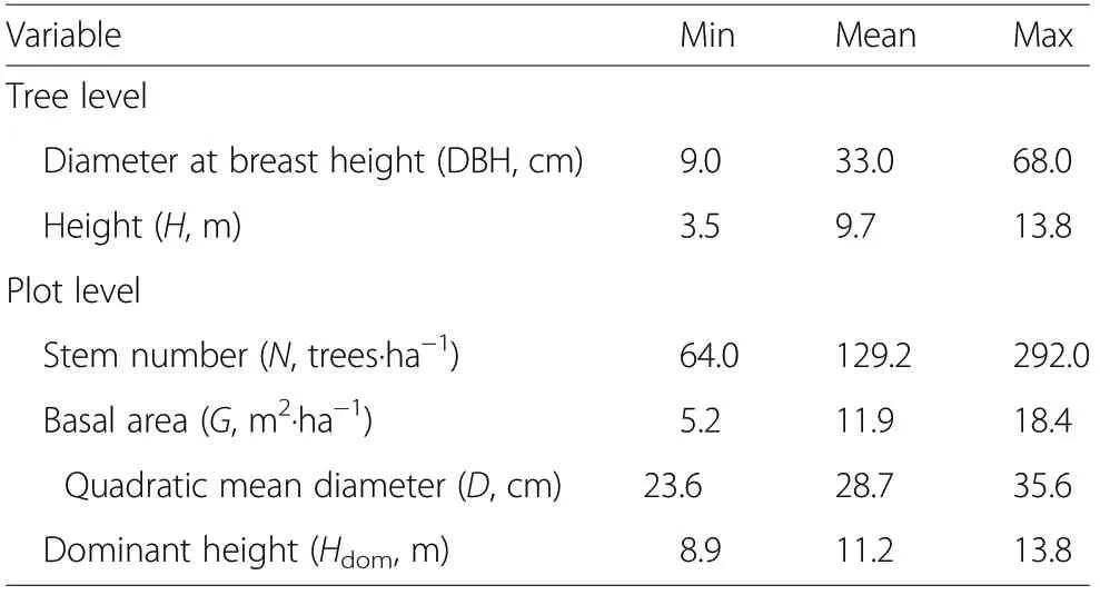
Table 1 Minimum, mean,and maximum of tree and plot attributes

Methods

Individual tree detection and tree attribute prediction

The canopy height model (CHM) of 1 m spatial resolution was interpolated by searching the highest ALS echo at AGL within each cell. If there were no ALS echoes within a cell, the value was interpolated from the neighboring cells. Individual trees were detected by searching treetops from the CHM. This was implemented with a local maximum filter (Hyypp? et al.2001). The CHM was slightly smoothed before searching local maxima to remove false positives (Koch et al.2006). Local maxima located ＜3 m (AGL) were removed in order to exclude local maxima on the ground and very small trees. Tree height was considered the same as the height (AGL) of the local maxima in the unsmoothed CHM. Tree detection worked quite well in the study area even though the ALS data had low echo density. The reason for this is that the crowns of individual stone pine trees do not usually touch each other.

The trees measured in the field plots and ALSdetected trees were linked to each other if treetops were located within a 3-m Euclidean distance in threedimensional space (see details in Vauhkonen et al. 2011).Then a tree diameter model was fitted using successfully linked trees as follows:

where DBH is the diameter at breast height in the fieldmeasured tree, HALSis the ALS detected tree height, and β0and β1are coefficients estimated from the data. We fitted the model with the least squares method using the nls function available in the R environment (R Development Core Team 2011). The estimated model coefficients (β0=5.3602, β1=2.2675) were statistically significant with both p-values less than 0.001.The coefficient of determination (R2) of the model was 0.66 and the RMSE was 5.26 cm. Finally, the model was used to predict DBH for all detected trees in the study area. The outputs of the ITD inventory were tree coordinates(XY), height and DBH for all detected trees.

Growth and yield models

The models presented in Calama and Montero (2006)were used to calculate the stem volume using predicted tree height and DBH for all trees. For each detected tree,the number of trees per hectare, basal area and dominant height (mean height of 100 largest trees per hectare)were computed using a buffer of 20 m around the tree.Site index was calculated using the existing model of Calama et al. (2003). The stand age in the study area was 78 years. The taper model (Calama and Montero 2006) was used to calculate the value of the stem. The following assortments, top diameters (dtop), minimum log lengths (hmin) and unit prices were assumed (Pasalodos-Tato et al. 2016): grade 1 (dtop≥40 cm, hmin2.4 m,30 €·m-3), grade 2 (dtop≥30 cm, hmin2.4 m, 18 €·m-3),grade 3(dtop≥20 cm, hmin2.4 m,13 €·m-3),grade 4 timber (dtop≥5 cm, hmin1.0 m, 5 €·m-3). The models from Calama and Montero (2004, 2005) were used to predict the 5-year increment in DBH and tree height, and the taper model was again used to compute the volume and the value of the trees 5 years later. Value increment was obtained as the difference of stem value at two time points. The relative value increment over a period of 5 years was calculated by dividing value increment by the value of the stem in the beginning of the 5-year period.See Pasalodos-Tato et al. (2016) for more details.

A power diagram to create tree regions

Tree-level forest data consist of detached tree regions(i.e. tree crowns) or points (i.e. stem locations), but not adjacent regions (e.g. grid cells or stands). Here we consider trees as point type objects. Then, we partition the space to trees with the assumption that a large tree occupies a larger area than a small tree. We refer to these partitions as tree regions. The partitioning is based on a power diagram, which is a type of weighted Voronoi diagram (Aurenhammer 1987). The power diagram is defined from a set of circles. Circle center is called a site.In this study, detected tree locations are sites and predicted DBH multiplied by 50 defines the radius of each circle. The power diagram consists of the points with the smallest power distance for a particular circle. In the case where all the circle radii are equal, the power diagram coincides with the Voronoi diagram. An example of the power diagram is given in Fig.2. Tree regions enable the use of adjacency relationships that take into account tree size, and the spatial optimization can be performed in a similar way as employed with traditional regions (e.g. grid cell or stand).

Spatial optimization

The cellular automaton developed for this study follows the ideas presented in Heinonen and Pukkala (2007) in which both local and global objectives are included in the priority function. In this study, the following priority function P was maximized for each tree:

where VTreeis the volume of the subject tree (m3), VTotalis the volume of all trees within the optimization area,RelValInc is the relative value increment of the tree (%in 5 years), CC is the proportion of the cut-cut border(of the total border length with adjacent tree regions;Fig.3); CuC is the proportion of the cut-uncut border;w1, w2and w3are the weights of the “l(fā)ocal” tree-level objectives RelValInc, CC and CuC, respectively; p1, p2and p3are sub-priority functions of the local objective variables (Fig.4); w4is the initial weight of the “global”objective TotCut (total volume of cut trees) and p4is a priority function for the global objective. In this study,the proposed target volume to be harvested was 20% of the initial standing volume. The target harvest was 654.6 m3for Area #1 and 459.3 m3for Area #2.

The priority function of Eq. 2 can be interpreted as a removal score for a tree. Low relative value increment(high economic maturity) and presence (aggregation problem) or absence (dispersion problem) of cut neighbors increases the probability of removal. Maximizing CC leads to the aggregation of cut trees and a large total area of cut trees, while the minimization of CuC contributes to compact aggregations on cut trees (Heinonen and Pukkala 2004).

In the CA developed in this study, two options were inspected for every tree for several iterations:cutting the tree or letting it continue to grow. The option that maximizes the priority function was selected. All trees were inspected during each iteration in random order. After a certain number of iterations,the weighting of the global objective variable (w4) was progressively incremented using a certain step. Iterations with gradually increasing value for w4were repeated until the total volume of harvested trees was sufficiently close to the target value of harvested volume. In this study, the initial value of w4in the optimizations was always 0.01. Three iterations were conducted with the initial value, after which the value of w4was incremented by 0.01 after every additional iteration. Iterations were stopped when the difference between the achieved harvested volume and the target volume was less than 5% of the target removal.

The CA described above is a simplified version of the automaton proposed by Strange et al. (2002) and Heinonen and Pukkala (2007). The first simplification is that the innovation probability is constant (one),implying that all trees are inspected at every iteration.The second simplification is that there are no mutations (mutation probability is constantly zero). Previous studies have shown that a high innovation probability and a low mutation probability work well in forest management problems (e.g., Heinonen and Pukkala 2007).

The CA described above leads to aggregations of cut trees. If the aim is to disperse cut trees, CC needs to be minimized and CuC maximized.In that case, the priority functions for CC and CuC need to be replaced by a 1-0 and 0-1 sub-utility functions, respectively, as shown with dashed lines in Fig.4. The following weights were used to mimic the various silvicultural tree selection methods in optimization:

· Non-spatial: RelValInc (w1=0.99), CC (w2=0.00),CuC (w3=0.00), TotCut(w4=0.01 initially)

· Single tree: RelValInc (w1=0.84), CC (w2=0.05),CuC (w3=0.10), TotCut(w4=0.01 initially)

· Tree group: RelValInc (w1=0.79), CC (w2=0.05),CuC (w3=0.15), TotCut(w4=0.01 initially)

· Clearcut:RelValInc (w1=0.69), CC (w2=0.10),CuC (w3=0.20), TotCut(w4=0.01 initially)

In the Single tree selection,the aim was to disperse trees,which was achieved by using the sub-priority functions for CC and CuC shown as dashed lines in Fig.4. In the Tree group and Clearcut selections, the aim was to aggregate trees, which was achieved by using the sub-priority functions for CC and CuC shown as continuous lines in Fig.4.

Results

Initial tree regions

The number of tree regions in Area#1 and Area#2 was 13,438 and 4296, respectively. The tree regions, together with tree volume and relative value increment of the tree, are shown in Fig.5. Tree spacing and consequently the size of tree regions differed between areas.The size of tree regions was smaller in Area #1 (mean 73, range 6-279 m2) than in Area#2(mean 98,range 10-938 m2).In general,trees were much larger in Area #2 (mean 0.49 m3, max 1.70 m3per tree)than in Area#1(mean 0.26 m3,max 0.72 m3per tree).The relative value increment (% in 5 years) was almost equal in both areas but due to larger trees the value increment(€in 5 years)was substantially higher in Area#2.

There was a clear east-west gradient in relative value increment in Area #2. This was partly due to small trees that rapidly increased their value but was also due to the higher site index (data not shown here) in the western part of Area #2. The relationship between tree volume and relative value increment was apparent: low tree volume indicated high relative value increment, which is logical due to the rapidly increasing proportion of valuable timber assortments in small trees.

Effect of tree selection method on stem number, tree size and value increment

In the absence of spatial objectives (Non-spatial), the proportion of cut trees (Table 2) and the relative value increment of those trees (Table 3) were less than in cases where spatial objective variables were included.

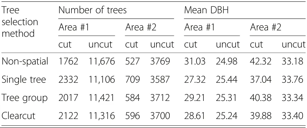
Table 2 Effect of tree selection method on the number of trees and mean diameter at breast height (DBH)for cut and uncut trees

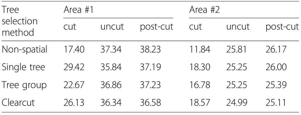
Table 3 Effect of tree selection method on the relative value increment (%in 5 years)for cut, uncut and post-cut trees

The difference between Non-spatial and Single tree selections was clearly evident: aiming for dispersed locations of cut trees increased the average relative value increment of cut trees by almost 70%. This means that the dispersion objective led to the removal of trees that were not among the most economically mature. In both areas, the inclusion of spatial objective variables slightly decreased the average DBH of the cut trees.

In Tree group and Clearcut the purpose was to aggregate cut trees.The relative value increment of cut trees increased more (compared to Non-spatial) when more weighting was given to aggregating harvested trees,meaning that large cutting aggregations led to the removal of many economically productive trees. Logically, the difference in relative value increment between cut and uncut trees decreased with increasing importance of creating cutting aggregations. In Area #2, the relative value increment of cut trees was greatest with Clearcut, whereas the Single tree method in Area#1 clearly resulted in the greatest relative value increment of cut trees.This suggests that Clearcut in Area#2 and Single tree in Area#1 were most in conflict with the economic objective.

The relative value increment was also computed after simulating the removal of the selected trees. The relative value increments were calculated with the assumption that the cut trees no longer existed in the stand.We call this the"post-cut" stage (Table 3). In general, the post-cut values were slightly greater than the uncut values. The difference in uncut and post-cut values was greatest in Single-tree selection and smallest in Clearcut selection, because Single tree selection decreased the competition of almost all trees,whereas the competition in Clearcut was decreased only for trees that were growing near the edges of the cut areas.

Size and spatial distribution of harvest blocks

The number of harvest blocks (continuous tree regions selected for cutting) was 4-5 times greater in Single tree than in the Non-spatial tree selection method (Table 4).Correspondingly, the mean size of the harvest blocks was about three times smaller in Single tree than in the Non-spatial selection method. Moving from the Nonspatial to the Tree group method increased the mean size of harvest blocks 8- or 9-fold. The Clearcut selection, which had a higher weighting on spatial objectives,clearly provided the largest harvest block size and the smallest number of harvest blocks.

On average, the distance from a cut tree to the nearest cut tree was longest with the Single-tree selection method (Table 5). This proves that Single-tree selection performed as desired (the purpose was to disperse cut trees). In the Non-spatial selection, the mean distance between cut trees was shorter than with the Single-tree selection and the standard deviation of distances was greatest. This is a logical outcome because Non-spatial selection does not attempt to generate a particular spatial distribution of trees.In the Tree group and Clearcut selections, the distances of cut trees were shortest because the aim was to cluster cut trees. The mean distances from uncut trees to their nearest neighbors were also shortest in the Tree group and Clearcut where most of the area was not thinned at all. Compared to cut trees, however, the mean distances did not vary much between tree selection methods.

Maps showing the spatial pattern of harvest blocks and the tree regions are displayed in Fig.6(Area #1) and Fig.7 (Area #2). Visual inspection verifies the conclusions drawn from Tables 4 and 5: (a) the Non-spatial selection does not show any particular spatial layout, (b)the Single-tree selection disperses trees to be cut, (c) the Tree group and (d) Clearcut selections cluster cut trees to various degrees, Clearcut more than Tree group. The spatial distribution of cut trees is slightly different in the two areas. In Area #1, where the spatial distribution is somewhat regular, the Single-tree method selected trees to be cut more evenly than in Area #2, where trees grow more in groups and stand density and tree spacing is variable.

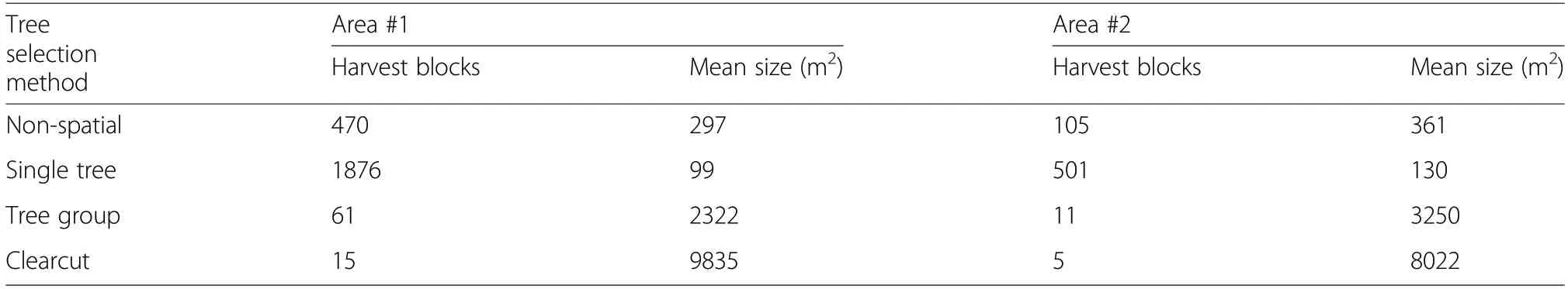
Table 4 Number of harvest blocks(i.e., continuous tree regions selected for cutting) and mean size(m2) of blocks

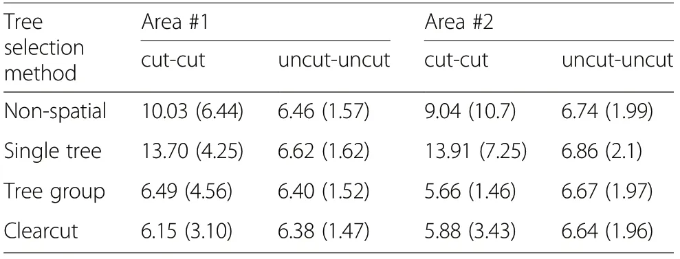
Table 5 Mean distance between trees and their nearest neighbors.

Discussion

We presented a new approach for tree-level harvest planning that considers both the spatial distribution and the value increment of the trees. The problem is formulated as a multi-objective optimization problem, which is solved by a tailored CA algorithm. The idea is to bundle the tree selection method with tree-level inventory data obtained by means of ITD and ALS data. The ITD inventory is currently a feasible method for certain forest types in an operational setting.Therefore,there is a need to develop spatially explicit methods for tree-level harvest and forest planning.

Spatial optimization in the forestry context is typically based on adjacency relationships of region type objects (Weintraub and Murray 2006). In practice, adjacency is often defined by computing cut-cut and cut-uncut border lengths of adjacent regions. Because tree-level data do not form adjacent regions, we partitioned the space to trees with the assumption that a large tree represents a larger area than a small tree.This means that both tree size and distance to its neighbors are included in the definition of adjacency:for large trees the length of the common border with adjacent trees is greater than for small trees. However, it is not apparent how strongly tree size should affect the size of the tree region. We used a power diagram to compose the tree regions, wherein the radius of a circle is the tuning parameter, the value of which depended on the tree size. We defined the radius of the circle to be 50×DBH. This value was selected arbitrarily, and future studies should examine the best approach to define its value more precisely.For example, the radius of a circle could be defined based on the growth potential of a tree.

Tree selection was combined with the use of an individual tree-level growth model that takes into account the neighborhood of the target tree. If tree selection requires the use of growth models, such as the relative value increment used in this study, it makes sense to use distance-dependent tree-level growth models or regular tree-level growth models in a spatial manner. Otherwise,the growth model predicts similar growth for all spatial distributions of trees and does not properly react to cuttings in the neighborhood of a target tree.

We controlled the spatial distribution of cut trees by modifying the weights and sub-priority functions of spatial objective variables CC and CuC. The weight of the global objective (total volume of cut trees) was fixed to a small initial value (0.01) in every case. The economic criteria (relative value increment) always received the remainder of the weights (1 - TotCut -CC - CuC). In the Non-spatial selection, the weights of CC and CuC were set to zero, thus the spatial aspect was ignored entirely (Figs. 5a and 6a). It provided a reference to other selections that took the spatial distribution of the trees into account. In the Single tree selection, CC was minimized and CuC was maximized. This clearly dispersed trees to be cut(Figs. 6b and 7b). In the Tree group selection, cutting aggregations were targeted with low weights for CC and CuC. This led to tree groups of different sizes(Figs. 6c and 7c). In the Clearcut selection, the spatial weights of CC and CuC were larger, which led to bigger tree groups resampling traditional clearcut areas(Figs. 6d and 7d). We deliberately used a rather simple priority function; there could be more objective variables and sub-priority functions. For instance, a constraint type sub-priority function could be used to force a certain size of tree groups.

Modifying the sub-priority functions and the weights of the spatial objective variables (CC and CuC) offers a means to enable the CA to mimic different disturbance regimes (Kuuluvainen 2016; Kulakowski et al. 2017),while always aiming at economically profitable forestry.For example, dispersion of cut trees (Single tree) mimics the damage caused by some insects that kill individual weak trees, the Tree group selection produces a landscape similar to wind damage (Kulakowski et al. 2017)and the Clearcut selection might correspond to damage caused by forest fire. Therefore, varying the weightings and sub-priority functions of spatial objective variables makes it possible to produce forested landscapes resembling those that result from different natural disturbance regimes.

In addition to disturbance regimes, it is also possible to mimic alternative silvicultural systems, ranging from continuous cover selection forestry (Single tree) via group selection (Wing et al. 2019) to evenaged forestry where clear-fellings are conducted in mature stands. The degree to which a certain disturbance regime or silvicultural system is pursued can be closely controlled. If low weights are given to the spatial objectives, the outcome of CA mainly depends on the heterogeneity of the forest. Large disturbances are created in forests where economically mature trees form large aggregations and tree groups are harvested when mature trees occur in groups. In this way, it is possible to mimic different disturbance regimes at minimal loss in profitability of timber production. A greater need to control the spatial aggregation of cut trees would increase economic losses.

In this study, we present and evaluate the proposed tree selection method as a tool for tree-level harvest planning. However, the method can be used as a part of a multi-objective forest planning system, in which dynamic treatment units are composed from trees by means of spatial optimization. This means that the trees to be cut are selected in each planning period, and subsequent periods must take into consideration the silvicultural operations implemented in earlier periods. The use of the proposed tree selection method as a part of multi-objective forest planning needs to be examined in subsequent studies.

Conclusions

The proposed tree selection method considers the spatial distribution of harvested trees and economic goals. It can be used to simulate cuttings in different type of silvicultural systems and mimic various disturbance regimes. It is easy to control by adjusting the sub-priority functions and the weightings of the spatial objectives. The method is utilized here as a tool in tree-level harvest planning but it can also be used in longer term forest management planning.

Abbreviations

ALS: Airborne laser scanning; ABA: Area-based approach; ITD: Individual tree detection; CHM: Canopy height model; AGL: Above ground level;DTM: Digital terrain model; DBH: Diameter at breast height; RMSE: Root mean square error; HALS: Height of ALS detected tree; CR: Circle’s radius in power diagram; CA:Cellular automaton;RelValInc:Relative value increment of the tree; TotCut: Total volume of cut trees; CC:Proportion of cut-cut border; CuC: Proportion of cut-uncut border; VTree: Volume of the subject tree; VTotal: Volume of all trees

Acknowledgements

The authors would like to thank Mr. Francisco Rodríguez from the ‘For? Forest Technologies’ for providing the field plot data to this study.

Authors’contributions

All authors contributed to the design and implementation of analysis.Authors also wrote the manuscript together,and all authors read and approved the final manuscript.

Funding

This research was supported by the University of Eastern Finland Strategic Funding, School of Forest Sciences and the Strategic Research Council of the Academy of Finland for the FORBIO project (Decision Number 314224).Adrián Pascual was also partially funded by Portuguese National Funds through FCT -Funda??o para a Ciência e a Tecnologia, I.P. in the scope of Norma Transitória - DL57/2016/CP5151903067/CT4151900586, and the project MODFIRE-A multiple criteria approach to integrate wildfire behavior in forest management planning with the reference PCIF/MOS/0217/2017.

Availability of data and materials

The tree regions and associated tree attributes used in the study are available from the corresponding author on reasonable request.

Ethics approval and consent to participate

Not applicable.

Consent for publication

Not applicable.

Competing interests

The authors declare that they have no competing interests.

Author details

1School of Forest Sciences, University of Eastern Finland, PO Box 111, 80101 Joensuu, Finland.2Forest Research Center, School of Agriculture, University of Lisbon, Tapada da Ajuda, 1349-017 Lisboa, Portugal.

Received: 11 September 2019 Accepted: 23 March 2020