Comparison of estimators of variance for forest inventories with systematic samplingresults from artificial populations

Steen Magnussen,Ronald E.McRoberts,Johannes Breidenbach,Thomas Nord-Larsen,G?ran St?hl,Lutz Fehrmann and Sebastian Schnell

Abstract

Keywords: Spatial autocorrelation, Linear trend, Model based, Design biased,Matérn variance, Successive difference replication variance, Geary contiguity coefficient, Random site effects

Introduction

Forest inventories have a long history of using systematic sampling (Spurr 1952, p 379) that continues to this date at both local, regional, and national levels (Brooks and Wiant Jr 2004; Kangas and Maltamo 2006; Nelson et al.2008; Tomppo et al. 2010; Vidal et al. 2016). Since forests exhibit non-random spatial structures (Sherrill et al.2008; Alves et al. 2010; von Gadow et al. 2012; Pagliarella et al. 2018), the main benefit of a uniform sampling intensity across a population under study (i.e. spatial balance) is an anticipated lower variance in an estimate of the population mean (total). However, the lack of a design-unbiased estimator of variance for the mean(total) remains a detractor (Gregoire and Valentine 2008,p 55).We do not have a design-unbiased estimator of variance for systematic sampling because the sampling locations are fixed by one independent random selection of a starting point and a sampling interval (d). With only one random draw, the systematic sample can be regarded as a random selection of one cluster with an undefined design-based variance (Wolter 2007, p 298).

Without a design-unbiased estimator of variance, it becomes a challenge to quantify the advantage of systematic sampling, and to compute reliable confidence intervals for estimated population parameters. The wide-spread use of a variance estimator for SRS without replacement (S?rndal et al. 1992, p 28) masks the advantage (efficiency) since this estimator tends to overestimate the actual variance (Wolter 1984; Fewster 2011). An overestimation that is, possibly, regarded as less problematic than an underestimation, and often referred to as a “conservative estimate”.

The bias in the variance estimator for SRS when applied to data from a single systematic sample was recognized early on in Scandinavian countries by Lindeberg(1924), Langs?ter (1926), and N?slund (1930), and in North America by Osborne (1942), and Hasel (1942).Lindeberg, Langs?ter, and N?slund also proposed new estimators of variance that generated more realistic estimates of variance for line-transect surveys (Ibid.). Variations of these estimators were later credited to others(Wolter 2007,ch. 8.2).

To convince an inventory analyst - with sample data collected under a systematic design - to employ an alternative to the estimator for SRS requires assurance that the alternative is nearly design-unbiased. That is, the expected value of the alternative estimator, over all possible (K) systematic samples from a finite population, is equal to or close to the variance among the K sample means (Madow and Madow 1944). Assurances of this kind will have to come from simulated systematic sampling from actual or artificial populations.

The lack of a design-unbiased estimator of variance means that any applied estimator is biased for the actual design variance (Opsomer et al. 2012; Fattorini et al.2018b). Variance estimators used in lieu of the design variance may carry the assumption that the sampling design is ignorable, or that any explicitly or implicitly stated model regarding the population is true (Gregoire 1998; Magnussen 2015). For example, when the estimator for SRS is applied to a systematic sample from a finite population, the design is ignored, and the variance is computed under the assumption that the sample values are independent.

In this study, we compare the performance of four alternatives to the estimator of variance for SRS in a suite of artificial populations with contrasting covariance structures and with or without a global linear trend. The performance in actual forest populations is deferred to a forthcoming study. The alternatives achieved - with respect to accuracy - a top ranking amongst 11 candidates in a preliminary study with 27 superpopulations described in Magnussen and Fehrmann (2019).

Although our primary focus is on systematic sampling designs with small populations (to expedite computations),and higher than practiced sampling intensities, we demonstrate that a ranking of the relative performances of estimators will be preserved in larger populations and a lower sampling intensity. We extend the same expectations to non-aligned and quasi systematic designs (S?rndal et al.1992, 3.4.2; Grafstr?m et al. 2014; Mostafa and Ahmad 2017;Wilhelm et al.2017),and possibly the random tessellated stratified design (Stevens and Olsen 2004; Fattorini et al.2009;Magnussen and Nord-Larsen 2019).

Materials and methods

Artificial populations

The four alternative estimators of variance are evaluated in realizations of two superpopulations: one (U1) with a stronger positive spatial autocorrelation between units in a single sample, and the other (U0) with a near zero spatial autocorrelation. Global linear trends (‘strong’,‘moderate’, ‘weak’, or ‘none’) are present in both U1 and U0. Populations without a linear trend are weakly stationary (Cressie 1993, p 53). An attractive estimator of variance will generate estimates that are close to the actual variance regardless of the strength of a spatial autocorrelation or the presence of a global trend. In practice,the effects of a significant trend can be mitigated by formulating a model (parametric or non-parametric) for the trend (Valliant et al. 2000, p 57; Opsomer et al.2012) or stratification (Dahlke et al. 2013).

The two superpopulations U1 and U0 are composed of N=57,600 equal size (area) spatial units arranged in a regular array with 240 rows and 240 columns. Edge effects is therefore not an issue in our study (Gregoire and Scott 2003). In an attempt to generate unit level autocorrelation in values of y compatible with forest structures, we generated random realizations (populations)U1, U2, …. from U1 and U0 with three additive random‘site’ effects (s1, s2, s3), operating at different spatial scales, plus unit-level random noise. The number of random spatial site effects is arbitrary. We know that forest attribute values depend on a multitude of factors operating at different spatial scales (Weiskittel et al. 2011). We consider three levels of site effects (e.g. soil, climate, and management) in our simulations of forest populations with a complex spatial structure.

To generate a site effect, the population under study was tessellated into a set of convex polygons (M?ller 1994). Then a site effect was assigned to each polygon by a random draw from a distribution specified for the site effect in question. All units with at least half their area in a polygon inherit the site effect of the polygon.The number, size, and centroids of polygons for a site effect varies from one realization of a superpopulation to the next according to random draws from distributions for the number and placement of polygons. A complete population was then composed of three spatial layers of polygon specific site effects (Fig.1), and one complete(240×240) layer of unit-level random noise.

Accordingly, the unit-level value yijin the ith row and jth column (i, j=1, …, 240) in a realization from a superpopulation is the sum of three random site effects s1, s2, and s3, a global trend τ, and random noise (e).We have

where sTij(T=1, 2, 3) is the random site effect associated with the polygon in which unit ij resides, τijis a unit specific trend effect, and eijis an independent random Gaussian noise. All units within a polygon share the site effect assigned to the polygon, which gives rise to a positive covariance among unit site effects within the polygon (Searle et al. 1992, ch. 11.2). To control the total variance in a study variable, the sum of site effects and random noise was standardized to a mean of zero and a variance of one. Technical details are deferred to the Additional file 1.

In addition to the spatial autocorrelation, we simulated three levels of a non-null global linear trend(Table 1) in addition to the simulations without a trend(τij=0 ?{i,j}).

Six random realizations of population values of yijwithout a trend are shown in Fig.2. They convey, as intended, a complex mosaic of the overlapping site effects. The visual resemblance of different realizations from a single superpopulation is low.

Sample-based maximum likelihood estimates of the autocorrelation function (acf, Anderson 1976, p 4) in the six populations in Fig.2 are given in Fig.3. One acf is shown for each of the possible samples under a given design. A considerable sample-to-sample variation is visible in some illustrations.

There is no variance heteroscedasticity in the simulated noise. To gauge its impact, we ran separate simulations with heteroscedasticity but only sketch the results in the discussion.

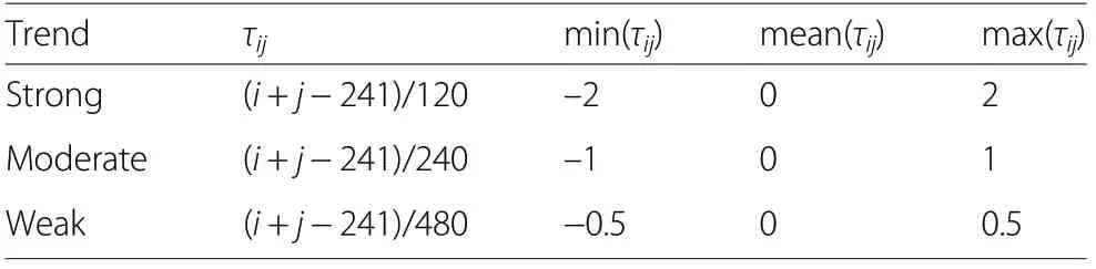
Table 1 Linear trend models and unit level trend components τij (i, j=0.5, 1.5,…, 239.5;cf. (1))

The population size in simulation studies are typically orders of magnitude smaller than actual finite populations.For the purpose of evaluating the relative performance of alternative variance estimators against a design variance,it is only important to stage:i)gradients of a spatial autocorrelation as done by choices of sample size; and ii) linear trends that will interact with sample size. A testing in a series of increasingly larger populations and across multiple spatial covariance structures is necessary if the relative performances of our estimators of variance are sensitive to sample size and/or trends. To assuage concerns about population size and sample size, we extended the simulations to include larger populations and a smaller sample size.

Sampling designs

Four systematic sampling designs are employed in the main study. Each design is defined by the sampling interval (d) in units in both of the two cardinal directions defining the population (here rows and columns)and a starting position (Cochran 1977, ch. 8.1; S?rndal et al. 1992, ch. 3.4.1; Fuller 2009, ch. 1.2.4). We have d=6, 8, 10, and 12. With a population matrix structure of 240 rows and 240 columns, the corresponding sample sizes were n=1600 (d=6), 900 (d=8), 576 (d=10),and 400 (d=12). We simulated all possible systematic samples (K) under a given design. The K starting positions by row and column were (di, dj), (di, dj)=1, …, d.Accordingly, K=d2or 36, 64, 100, and 144 for the designs with d=6, 8, 10, and 12. All K samples for a fixed sample size were executed and replicated 30 times, each time with K samples from a new random realization of a superpopulation (U1 or U0). Hence our results come from 2(superpopulations)×4(linear trends)×4(sample sizes)×30=960 random realizations (480 from U1 and 480 from U0). With 30 realizations from a superpopulation, the relative standard error of the mean of a design variance was approximately 3% for sample sizes 400 and 576, and 5% for sample sizes 900 and 1600.

A sampling design was implemented by selecting all possible (K) different (or non-identical) systematic samples under the given sampling interval d. Specifically, we first divide a 240×240 population into n =(240/d)2square blocks each with d rows and d columns. To select a single systematic sample, one would pick a random integer (k) from the set {1, …,K=d2) and then select one unit at position k from each of the n blocks. An example with d=6, and k=4 and k=20 is in Fig.4.

Note, Thompson (1992) defines a systematic sampling by primary and secondary sampling units. For designs with one primary unit and n secondary units, as the case is here, and in most natural resource surveys, we can,without consequence,dispense with the notion of primary sampling units, consider the secondary units as sample units,and take n as sample size(Thompson 1992,p 113).

Supplementary populations and sample designs

A population size of 240×240=57,600 is orders of magnitude smaller than the size of actual finite regional or national forest populations. Conversely, even a sampling intensity of n/N=400/57,600 or 0.7%is an order of magnitude greater than in practice. To augment the practical relevancy of our simulations, we gauged the impact of reducing the sample size to n=100 in trendless populations with a spatial autocorrelation and sizes N=57,600 unit (as in the main study), N=230,400 units in a 480×480 array, and N=921,600 units in a 960×960 array.The site effects were preserved at the levels detailed for the main study, but the number of polygons carrying a site specific effect was either defined as for the 240×240 unit populations in the main study, or doubled for N=230,400 units, or quadrupled for N=921,600 units. Thus the sample autocorrelation functions driving the variances will depend exclusively on the sampling interval (d=24,48,or 96),the size(number)of the site polygons and their overlaps. Results with the RIP estimator of variance were dropped in consideration of the time required to compute the results with this estimator.

Variance estimators

In accordance with the populations under consideration,the variance estimators considered are cast for finite populations composed of N units. For these populations under a given systematic design there is a finite number(K) of distinct (non-overlapping) samples. With minor modifications the estimators also apply to infinite (continuous) populations of sample locations (points), but here K=∞{Mandallaz 2008 #10986} and there is no finite population correction in the variance estimators.

Design variance

The design-based variance (DES) for systematic sampling in a finite population (Madow and Madow 1944)is

Variance estimator for simple random sampling

The SRS estimator of variance - when applied to a sample selected under a systematic design - ignores the actual (spatial) ordering of the sampled units, and, by extension, any covariance between these units. Let yidenote the ith unit in one of the K possible samples obtained under a systematic design. For a systematic sample of size n, taken from a population of N units, the estimator of variance is

Matérn’s estimator of variance

Matérn (1947) proposed a per point (i.e. local) estimator of variance inspired, in part, by the pioneering work of Langs?ter (1932), Langs?ter (1926), and Lindeberg (1924). These authors suggested the use of first- and second-order differences as a mean to reduce the effect of local trends resulting in autocorrelation (Wolter 2007, ch. 8.2.1.). To our knowledge, the Swedish and Finnish national forest inventories (NFI)were the first to adopt a variant of his estimator(Ranneby et al. 1987; Heikkinen 2006).

In Matérn’s estimator, the sample locations are split into Q non-overlapping groups of four nearest neighbours. An example is in Fig.5. Two predictions of the local mean are constructed for each group, and the squared difference of these predictions is taken as the per point variance.

With the notation in Fig.5,the two local predictions are computed as(yi,(j+1)+y(i+1),j)/2 and(yi,j+y(i+1),(j+1))/2.The final estimator of variance is the average per point variance. Modern parallels to this estimator can be found in texts on ordinary kriging (for example, Cressie 1989,ch. 3.2). Examples of practical applications with this estimator can be found in (Kangas 1993, 1994; Lappi 2001;Ekstr?m and Sj?stedt-de Luna 2004;Tomppo 2006).

In populations where a sample location can be outside the domain of interest (here forest), at least one sample location in each group must be in the domain. Computation of Matérn’s variance estimate is carried out with mean-centred values of yij. Within each group, the value of yijin locations outside the domain of interest is set to 0 (viz. the mean of all yijin the sample). We have(Matérn 1980, ch. 6.7, p 121; Ranneby et al. 1987)

where nqis the number of sample locations in a group in forest, and q ?{i,j} means that group q includes sample location {i, j}. Note, when all Q groups have four locations in the domain of interest, there is no need to mean-centre the observations. Conversely, the implicit imputation of the mean to location outside the domain of interest will, on average, inflate the variance in populations with autocorrelation.

Successive difference replication estimator of variance

The successive difference replication estimator of variance (SDR) was proposed by Fay and Train (1995). According to Fay and Train, SDR is an improvement over the first- and second-order difference estimators first proposed by (Lindeberg 1924) and later detailed in Wolter (2007). Like in a jackknife estimator of variance(Efron 1982),a number 2r-with r an integer and 2r-n-2 ≥0 - of pseudo-values of the sample mean is produced,and then the variance among these pseudo-values is taken as an estimate of the design variance in Eq. (1). For a sample size of, for example 400, we take r=9, and the number of pseudo-values becomes 512. Each pseudovalue is a weighted average of the n observations in a sample. To apply the SDR to a systematic sample from a spatial population, the sample units must be brought into an order compatible with a sample selected from a population with units arranged in a linear (one-dimensional)structure. SDR is applicable to a wide array of sampling designs(Opsomer et al.2016).

With our population units, identified by their row and column position in a grid, we applied the SDR estimator of variance with the n sample units ordered row-wise, column-wise, and to a shortest path (with start in the first sampled unit) through the n sample locations (Fig.6).

The simple average of the three SDR estimates of variance obtained with the row-wise, the column-wise, and the shortest path ordering of the sample is our SDR estimate of variance for a single systematic sample. The SDR estimator applicable to an ordered sample with r pseudo-values of the population mean is:

Ripley’s estimator of variance

Ripley’s estimator Ripley (2004) is model based and applies to a continuous (in y) population with infinitely many possible sampling locations (Mandallaz 2008, pp.60-62). Applied to a systematic sample of size n from a contiguous spatial area (A) equal to the extent of the finite populations under study, we have

We chose the distance-dependent covariance function for an isotropic weakly stationary fractional Gaussian noise process (FNG, Baillie 1996). FNG’s have been used to characterize ‘long-term’ memory processes (Johannesson et al. 2007; Nothdurft and Vospernik 2018). Accordingly, the covariance between observations from two units or two points separated by a distance h is

Computation of the last two terms in Eq. (6) can be demanding, in particular for large populations with an irregular spatial outline. In our computations we used Monte-Carlo integration (Robert and Casella 1999, ch. 5.3.2) over 2400 random points in A to obtain the second term on the r.h.s. of Eq. (6). To compute the third term on the r.h.s of Eq. (6) we exploited the fact that in a spatially continuous population with a simple geometric structure, we can integrate over all possible distances with a probability distribution function for the distance between two randomly selected points (Ripley 1977).

D’Orazio’s estimator of variance

D’Orazio’s estimator of variance (D'Orazio 2003) provides a correction (c) to the SRS estimator of variance intended to capture the effect of a spatial autocorrelation. The correction is through Geary’s contiguity ratio c - a measure of the spatial association between a sample unit value of y and the y-values in its nearest(spatial) neighbours (Geary 1954). Geary’s c takes a value of 1.0 when there is no association, while a c ＜1 suggests a positive spatial association, and a c ＞1 a negative association. The estimator showed promising results in a recent simulation study (Magnussen and Fehrmann 2019).

The idea behind D’Orazio’s estimator, hereafter referred to as DOR, is simple. From Eq. (2) it is clear that the desired design variance is the variance among the K sample means whereas the SRS variance in Eq. (3) is the within sample variance of a sample mean. Consider a breakdown of the fixed total variance in a (finite) population into a within- and between sample variance. With a positive (negative) spatial covariance among units in a population the among-sample variance will decrease (increase) relative to a population without a spatial covariance. This follows because the sum of the within-sample variance is inflated (deflated) by the covariance. Since the SRS estimator does not account for the within sample covariance, it requires a correction. D’Orazio opted to use Geary’s contiguity ratio as a correction factor since it represents an extension of the Durbin-Watson(DW) statistic (Durbin and Watson 1950) to a spatial context. The DW statistic was successful in explaining the apparent efficiency of nearest-neighbour poststratification in systematic sampling from populations arranged in a linear array (Ripley 2004, pp. 26-27). The DOR estimator of variance is

Monte-Carlo error in estimated variances

With 30 replications of K possible samples, the Monte-Carlo error (Koehler et al. 2009) on the average of an estimated variance was 4.6% (n=400) to 1.6% (n=1600) with the SRS estimator, 2.7% with the MAT estimator, 2.6% with the SDR estimator, and 1.2% (n=400) to 13.8% (n=1600) with the RIP estimator, and 2.4% with DOR.

Estimator performance

Results

Populations with autocorrelation and no trend

Results with D’Orazio’s estimator of variance in Fig.7 were nearly perfectly correlated with results from Matérn’s (0.992-0.995) and the SDR estimator (0.999-1.000) and therefore not detailed separately.

In terms of absolute deviations from the design-based variance, Matérn’s estimator was attractive when sample sizes were 400 and 576. In these settings, the average MAT estimate of variance - over the K samples - was in 17 (n=400) and 18 (n=576) out of 30 realizations of a superpopulation the least biased (Fig.8). With n=900,the MAT estimator was in 13 realizations the least biased, and Ripley’s estimator was 9 times the least biased. With the largest sample size (n=1600) RIP and DOR are the least biased in 11 and 10 realizations,respectively.

In terms of the distribution of absolute deviations,Fig.10 indicates a better anticipated performance of DOR and SDR with MAT as the runner up. RIP is a distant fourth and closest to the distribution provided by SRS.

Should an analyst prefer an estimator that has a variance that is not only at least 20% below the variance with SRS, but also not underestimating the design variance, the choice would again be SDR and DOR with an estimated probability of 0.45 and 0.48 for satisfying this criterion in our simulations. Corresponding results for MAT and RIP were 0.34 and 0.12.

Populations with autocorrelation and a linear trend

A global linear trend, unless accounted for by modelling or stratification, will increase the variance in sampled values of y. In the scenarios with a linear trend the SRS estimator of variance was again, by a wide margin, the most conservative of the five tested estimators (Table 2).The overestimation of variance increased rapidly with the strength of the linear trend, from 50% with a weak trend to 188% with a strong trend. Sample size (from 400 to 1600) had, in comparison, only a minor effect.Results with the MAT estimator were better. Its poorest performance was an overestimation of 19% in populations with a strong linear trend and a sample size of 400(d=12), in all other settings the estimated variance was within 4 percentage points of the design variance. The performances of SDR and DOR were similar but consistently lagged that of MAT, especially in the populations with a strong linear trend. The RIP estimator performed worse than MAT, SDR, and DOR in combinations of a strong or moderate trend and a sample size of 400. With a sample size of 1600 and a moderate or a weak trend,the performances of the four estimators MAT, SDR, RIP,and DOR were, from a practical perspective, similar.

Populations with near zero autocorrelation and no trend

In a population with a near zero autocorrelation, the proposed alternative estimators (MAT, SDR, RIP, and DOR) and the SRS should, ideally, generate estimates of variance close to the actual design variance (DES).As can be taken from Table 3, this was the case across all sample sizes and realizations of a superpopulation (hint: paired equal variance t-test p-values for the null hypothesis of no difference were all greater than 0.05). The applicability of the t-distribution was ascertained with a KS-test (Kolmogorov-Smirnov, P ＞0.34, Barr and Davidson 1973). We failed in all cases to reject the null hypothesis of a tdistribution.

Populations with a near zero autocorrelation and a linear trend

In populations with a near zero autocorrelation and a linear trend, the SRS estimator of variance was consistently the most conservative(Table 4)with an overestimation that increased with sample size and strength of a linear trend.Estimates obtained with MAT, SDR, RIP, and DOR were all closer to the actual design variance than the SRS estimates of variance,but with a distinct sensitivity to the interaction between sample size(sampling interval)and strength of the linear trend. With n=1600 the four alternative overestimated the actual variance by 22%-24%, but with n=400 the MAT, SDR, and DOR estimator underestimated the variance by 1% to 5%, whereas RIP overestimated the design variance,most(22%)in presence of a strong trend,and least(2%)with a weak trend.

Scaling to larger populations and a smaller sample fraction

With the results from the supplementary populations and sample designs we gauge the scalability of the results from the main study in Table 5. DES and SRS variances were almost constant across the three population sizes (57,600; 230,400; and 921,600), as predicted by theory. Variances obtained with MAT, SDR,and DOR were in all cases closer to the estimates of design variance than were the variances obtained with SRS. MAT was in each case closest to the DES variance but with a standard deviation across realizations almost twice as great as the standard deviation with DES. We also note that as the population size increased and the sample fraction decreased, the variances obtained with MAT, SDR, and DOR drifts - at a slow rate - towards the results of SRS. The DOR estimator has a much smaller standard deviation than MAT and SDR, suggesting that in even larger populations and smaller sample sizes, this estimator may, on a single-sample basis, frequently outperform MAT and SDR.

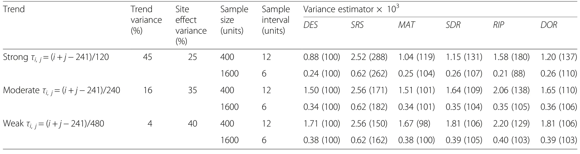
Table 2 Estimated variances in populations with spatial autocorrelation and a strong, a moderate, and a weak global linear trend.All table entries are means across 30 realizations of a super-population with autocorrelation and a linear trend,and the K possible sample for a given sampling interval(d).Variances in parentheses are relative variances with the DES variance fixed at 100.τi, j is the trend component for unit in row i and column j(i,j=0.5, 1.5,…, 239.5)

Discussion

Although we have a general methodology for constructing a model-based estimator of variance for systematic sampling that is model unbiased with a minimum root meansquared error (Wolter 2007, ch. 8.2.2), and we appreciate Tobler’s first law of geography (“units separated by a shorter distance are, on average, more similar than units separated by a longer distance”, Tobler 2004), we are still evaluating model-based variance estimators for systematic sampling (McGarvey et al. 2016; Strand 2017; Magnussen and Fehrmann 2019) or proposing new ones (D'Orazio 2003; Clement 2017; Pal and Singh 2017; Fattorini et al.2018a; Magnussen and Fehrmann 2019). A century long occupation that appears to have begun with the efforts by Lindeberg(1924)and Langs?ter(1932).

Table 3 Paired t-tests under the hypothesis of equal variances.is the difference between the mean estimate derived with SRS,MAT, SDR,RIP, or DOR and the design based variance (DES).is the absolute value of the t-statistics(effect size), and P(｜Δ =0) is the probability of a greater under the null hypothesis of a zero difference

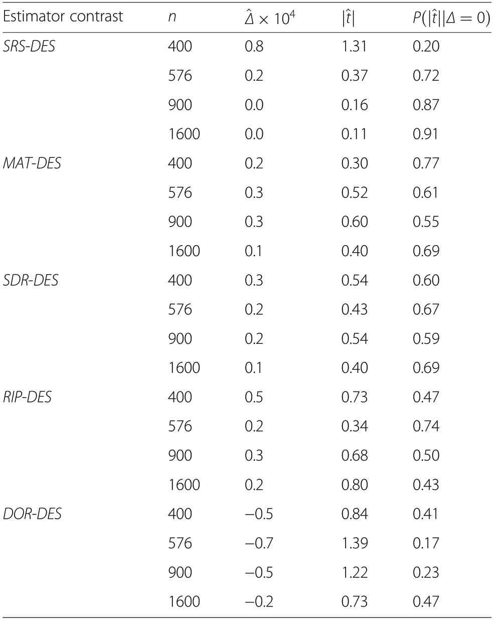
Table 3 Paired t-tests under the hypothesis of equal variances.is the difference between the mean estimate derived with SRS,MAT, SDR,RIP, or DOR and the design based variance (DES).is the absolute value of the t-statistics(effect size), and P(｜Δ =0) is the probability of a greater under the null hypothesis of a zero difference

Estimator contrastn^Δ×104｜^t｜P(｜^t｜｜Δ =0)SRS-DES4000.81.310.20 5760.20.370.72 9000.00.160.87 16000.00.110.91 MAT-DES4000.20.300.77 5760.30.520.61 9000.30.600.55 16000.10.400.69 SDR-DES4000.30.540.60 5760.20.430.67 9000.20.540.59 16000.10.400.69 RIP-DES4000.50.730.47 5760.20.340.74 9000.30.680.50 16000.20.800.43 DOR-DES400-0.50.840.41 576-0.71.390.17 900-0.51.220.23 1600-0.20.730.47

There is a simple explanation as to why a single omnibus estimator for systematic sampling is unlikely to emerge, and that is the sensitivity of the design variance to a non-random ordering of the population units (S?rndal et al. 1992, ch. 3.3.4). In forestry, we may have numerous non-random structures in any population of forest trees and associated vegetation that directly influence a study variable (Burslem et al. 2001; Scherer-Lorenzen and Schulze 2005). Spatial autocorrelation is just one of many manifestations of a non-random ordering, but it is pivotal for computation of variance in a spatial population.

The sensitivity of the design variance to a non-random ordering of population units calls for caution when we,from simulation studies, attempt to infer the performance of a variance estimator in a population with an unknown ordering. In particular when an estimator explicit or implicitly assumes a particular model for the study variable. Since “all models are wrong, but some are useful” (Box 1976), it is risky to assume that a model is true(Wolter 2007,p 305).

Yet, simulated systematic sampling from artificial or actual populations remains the most expedient method to screen variance estimators for systematic sampling.By necessity artificial populations will be simpler and smaller than actual ones. Ultimately, however, it is the spatial covariance structures in a population that drive the performance of a variance estimator (Fortin et al.2012). Casting the covariance process as the outcome of shared random effects is consistent with Tobler’s first law of geography (Tobler 2004). With autocorrelation arising from three additive site effects - of different strength and operating at three spatial scales - our populations are one step closer to resemble actual forested landscapes than possible with a parametric spatial covariance model (Wolter 2007, ch. 8.3; Magnussen and Fehrmann 2019). A different approach was taken by Hou et al. (2015). They generated spatial covariance structures by manipulating the spatial distribution of live trees in an actual plantation. In terms of the sampling distribution in estimated means, their approach delivered results consistent with ours. A nearly constant relative performances of the five estimators of variance, in populations of different size and more realistic sample fractions, vouch for the scalability of our findings and main results.

Table 4 Estimated variances in populations with a near zero autocorrelation and a strong, a moderate,and a weak global linear trend.All table entries are means across 30 realizations of a super-population and the K possible samples for a given sampling interval(d).Variances in parentheses are relative variances with the DES variance fixed at 100.τi, j is the trend component for unit in row i and column j(i, j=0.5,1.5…, 239.5)

Regional trends are commonplace in large-area forest inventories as they include sites with different climates,soils, species,forest structures, and associated forest management practices. If regional trends are not dealt with through modelling or a (post) stratification, they may drastically change the estimate of variance (Matérn 1980,ch. 4.6; S?rndal et al. 1992, p 82; Breidt and Opsomer 2000;Wolter 2007,Table 8.3.1).Our results with a strong,moderate,and weak global linear trend confirmed the sensitivity of the design variance to such trends. Each of the K sample means will differ by an amount determined by the average difference in y between adjoining population units.Regardless of the strength of a global trend,the four tested alternative variance estimators generated variances that were closer to the design variance than possible with the SRS estimator of variance. The MAT estimator is, in theory, robust against a unidirectional trend, but not against our bi-directional trends. In populations with a suspected trend, and no attempt to address the trend by modelling or a stratification, the MAT estimator emerged as most attractive followed by DOR and SDR. In larger populations, the less variable DOR estimator becomes more attractive. To be successful in populations with a trend,the RIP estimator requires a separation of trend and spatial covariance structures, otherwise the performance will be less predictable and more variable.

Heteroscedasticity is commonplace in data from actual forest inventories, but not included in our study settings.To gauge it importance, we ran simulations with a noise variance that increased linearly by a factor 3 across both rows and columns, and sample sizes 400 and 1600. The results (not shown) were similar to the results in Table 4 for a moderate trend and a near zero autocorrelation.That is, SRS was the most conservative with anoverestimation of variance of 40% (n=400) and 22% (n=1600), and MAT was the estimator with the performance closest to that of the target design variance (i.e. an overestimation of 10% for n=400, and an underestimation of 6%for n=1600).SDR was in this regard the runner up.

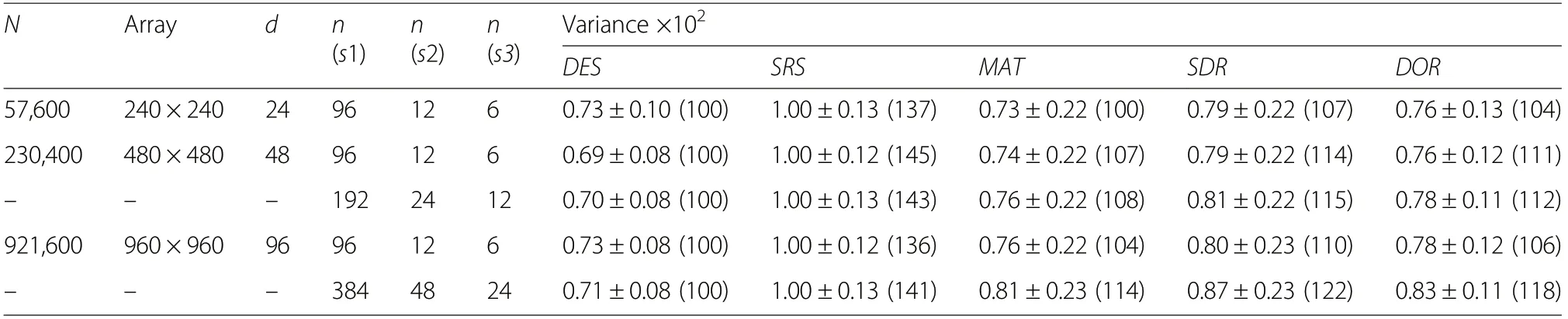
Table 5 Estimated variances with a systematic sample size of n=100 in trend-less populations with autocorrelation,scaled sizes (N),and scaled expected number of site polygons (n(sT),T=1,2,3). All results are based on 30 realizations of a superpopulation, and all or a maximum of 2000 random selections of all possible samples under a systematic sampling design. The standard deviation (^σ)across realizations is indicated(±^σ). Relative variances with DES fixed at 100 are in parentheses

Despite marked differences in formulation of the MAT, SDR, RIP, and DOR estimators of variance, their expected performance was quite similar in populations without a global trend. The strong correlations among the variances obtained under these conditions, confirms the importance of a first-order autocorrelation since it alone was captured by all four.Higher order autocorrelations enters only in the SDR and RIP estimators.

The MAT estimator had the lowest expected absolute bias, i.e. the lowest expected risk of over- or underestimating the actual variance. Yet, in practical applications MAT will be sensitive to edge effects. In a fragmented forest landscape, its performance may suffer.The expected performance of DOR and SDR was close to that of MAT. From a practical perspective there is no strong rationale for preferring one over the other in populations with either no trends or with a trend dealt with through modelling or stratification. Otherwise the MAT estimator followed by SDR and DOR can be recommended.

The expected performance of RIP was sensitive to trends and varied with sample size which makes recommendations to practice more difficult. The sensitivity to sample size is largely a question of the number of integration points for computing the second term in Eq. (6).With 9600 integration points the performance was nearly constant across sample sizes (not shown), but with this number of integration points the computation time became impractical. Moreover, computational challenges in applications with large populations and a fragmented forest landscape, may further detract from its appeal in terms of supportive theory in spatial statistics(Thompson 1992, ch. 21; Ripley 2004).

In populations with a very weak autocorrelation, all estimators reproduced the design variance with a low margin of error. Thus, the risk of a counter-factual or a spurious result appears to be low with the four alternative estimators of variance.

In terms of the anticipated performance in a single application (without trends), the DOR and SDR estimators generated a higher frequency of estimates closer to the design variance than estimates from MAT and RIP.Moreover, DOR and SDR were also best in terms of the odds of generating a variance estimate that is at least 20% below the SRS without underestimating the actual variance.

DOR has two advantages over SDR, it is computationally simpler, and it provides a metric (Geary’s c)of the first-order spatial correlation (association). The magnitude and sign of Geary’s c provides a useful and interpretable statistic. It is fairly straightforward to implement a spatial randomization of the sample locations and repeat the estimation of Geary’s c a large number of times to obtain the distribution of c under the null hypothesis of no spatial association amongst first-order neighbours. A rejection of the null hypothesis serves to argue against the SRS variance estimator.

As suggested from the supplementary yet limited simulations with larger populations (without a trend) and lower sample fractions, the estimates of variance obtained with the five estimators will gradually converge as N increases and n/N decreases. This was expected since d is inverse proportional to n/N and the average autocorrelation typically declines with an increase in d.

Several estimators of variance tailored to semisystematic sampling (Stevens and Olsen 2003; Magnussen and Nord-Larsen 2019), quasi-systematic sampling(Wilhelm et al. 2017), or designs with a spatial balance in auxiliary space (Grafstr?m et al. 2014) were beyond the scope of this study. Given the model-based nature of MAT, SDR, RIP, and DOR, we expect they will be of interest also for these variations on systematic sampling.

We made no use of auxiliaries from remote sensing although they are omnipresent. As pointed out by Opsomer et al. (2012) and Fattorini et al. (2018a) “… for a model that fit the data well, any variance estimation method that targets the residual variability will perform satisfactorily regardless of the autocorrelation in the sample data”. In the forerunner to this study (Magnussen and Fehrmann 2019), we confirmed that the conservative nature of the SRS estimator of variance diminishes with the strength of the correlation between y and an auxiliary variable (x).

All our results apply to finite populations considered as realizations of a superpopulation (Bartolucci and Montanari 2006). We could have employed the infinite population paradigm on the finite-area populations under study with the constraint of equality in size (area)of a population unit and a sample plot. We would, in theory, have an infinite number of possible samples for a fixed sample size, but if we excluded samples with edgeeffects and samples with overlapping plots - which violates the strong assumption of independent samples -we would generate results very similar to those presented.

We recognize that an analyst, accustomed to application of the SRS estimator of variance to data obtained under a systematic sampling design, may not be swayed by results from simulations or simulated sampling from actual populations. Yet, to continue with the SRS without an attempt to gauge the need for an alternative is not best practice. With today’s powerful computers and readily available software for spatial analysis, it is not difficult to obtain statistics to guide an analyst towards a suitable estimator of variance. While issues of trend and heteroscedasticity may be addressed with a modelling,post-stratification (D'Orazio 2003; Westfall et al. 2011;Strand 2017; McConville and Toth 2017; Magnussen and Fehrmann 2019) or the one-per-stratum design proposed by Breidt et al. (2016), the issue of autocorrelation will persist across spatial scales.

Conclusions

The conservative nature of the SRS estimator of variance when applied to data collected under a systematic design was confirmed. The provision of conservative estimates of variance is counter-productive in an era where forest resource estimates are increasingly important in a number of policy issues where precise estimates are expected.Inflated estimates of variance may obscure opportunities for cost-savings from reduced sampling efforts that do not imperil targets set for precision. Additional computational complexities are encountered when switching from the SRS estimator to a better alternative, but they are not necessarily dissuasive.

In populations with spatial autocorrelation,the four alternative estimators of variance generated estimates of variance that were much closer to the actual design variance than possible with the SRS estimator. In the populations with near zero spatial autocorrelation the four alternatives closely tracked the actual design variance.No single alternative estimator emerged as uniformly best in terms of bias. In terms of expected performance in populations without a trend, MAT was slightly better than SDR and DOR. In terms of the anticipated (single sample) performance, DOR and SDR emerge as less variable than MAT. In populations with a strong or a moderate global linear trend, we would recommend MAT.Nevertheless, in a large population and a low sampling intensity,the performances of the investigated estimators will be less distinct.

Supplementary information

Supplementary information accompanies this paper at https://doi.org/10.1186/s40663-020-00223-6.

Acknowledgements

Two anynomous reviewers made many constructive suggestions to improve our first submission.Their help and support are greatly appreciated.

Authors’ contributions

The first author conceptualized and executed the simulations, obtained and analyzed the results, and wrote a first draft of the manuscript. Subsequent authors (2 to 7) participated in discussions around study design, populations,estimators, and made improvements to the first draft of our manuscript. The author(s) read and approved the final manuscript.

Funding

No external funding provided.

Availability of data and materials

The datasets used and/or analysed during the current study are available from the corresponding author on reasonable requests.

Ethics approval and consent to participate

Not applicable.

Consent for publication

Not applicable.

Competing interests

The authors declare that they have no competing interests.

Author details

1506 West Burnside Road, Victoria, BC V8Z 1M5, Canada.2Raspberry Ridge Analytics, 15111 Elmcrest Avenue North, Hugo, MN 55038, USA.3Norwegian Institute of Bioeconomy Research, H?gskolevegen 8,1431 ?s, Norway.4Department of Geosciences and Natural Resource Management, University of Copenhagen, Rolighedsvej 23, DK-1958 Frederiksberg C, Denmark.5Department of Forest Resource Management, Swedish University of Agricultural Sciences, Ume?, Sweden.6Forest Inventory and Remote Sensing,Faculty of Forest Sciences, University of G?ttingen, Büsgenweg 5,D37077,G?ttingen, Germany.7Alfred-M?ller-Stra?e 1,Haus 41-42, 16225 Eberswalde,Germany.

Received: 6 November 2019 Accepted: 26 February 2020