Numerical accuracy and convergence with EMC3-EIRENE

Kristel GHOOS,Heinke FRERICHS,Wouter DEKEYSER,Giovanni SAMAEY and Martine BAELMANS

1 KU Leuven,Department of Mechanical Engineering,B-3001,Leuven,Belgium

2 University of Wisconsin Madison,Department of Engineering Physics,WI 53706,United States of America

3 KU Leuven,Department of Computer Science,B-3001,Leuven,Belgium

4 Author to whom any correspondence should be addressed.

Abstract

Keywords:convergence,Monte Carlo,numerics,plasma edge,EMC3-EIRENE

1.Introduction

The coupled Monte Carlo–Monte Carlo (MC–MC) code EMC3-EIRENE [1,2]is developed to enable plasma edge simulations in complex,3D geometries as present in stellerators such as W7-X and W7-AS.It has also been applied to study 3D phenomena in tokamaks,including ITER [3,4].EMC3 solves a simplified version of the Braginskii fluid equations by means of a MC method [5].Stochastic differential equations are derived to model the evolution of the particle properties.The domain is divided into a number of cells in which quantities of interest (density,velocity,temperatures) are estimated based on particle trajectories.MC particles are followed using small time steps with corresponding random walks,where convective and diffusive processes are taken into account [6].The main advantage of this method is its high flexibility in the construction of the computational mesh.EMC3 is often coupled to the MC code EIRENE [2],which is used to solve a Boltzmann-type equation for neutral particles in 3D space.

The EMC3-EIRENE code system is solved for steadystate problems by iterating both codes alternately until the relative change in the solution is typically ≤1% [7].It is assumed that this value is a measure of the statistical error on the solution.It has been demonstrated,however,that this stopping criterium is insufficient as an error estimate since the relative change can give a misleading indication and neglects deterministic error contributions[8].Deterministic errors arise from solving nonlinear problems with a finite number of MC particles (bias),advancing fluid MC particles with a discrete time step (time integration error),and using discretized variables in space (discretization error).

Each deterministic error contribution can be estimated based on the theoretical error reduction rates by comparing solutions with a different grid resolution,time step,or number of MC particles per iteration.By varying the time step,the number of MC particles per iteration or the grid size,the magnitude can be estimated for respectively the time integration error,the bias and the discretization error.To obtain reliable estimates,it is important to have a sufficiently low variance on the solutions,which can be efficiently obtained by using post-processing averaging.This does not only enable accuracy analysis,but can also significantly reduce the required CPU-time.This error estimation strategy and simulation approach has been used previously to study the accuracy for B2-EIRENE simulation of a partially detached ITER divertor plasma[9].In B2-EIRENE,only EIRENE is an MC code,while B2 is a deterministic,finite volume code.

In this paper,we analyze the different numerical error contributions for an EMC3-EIRENE simulation of an axisymmetric DIII-D divertor edge plasma.After a short case description in section 2,the simulation approach is explained,where post-processing averaging is introduced in section 3.Afterwards,we discuss the error reduction rates for the time integration error,bias and statistical error for simulations where only one module,the EMC3 energy module,is solved in section 4.Subsequently,we investigate the accuracy in a fully coupled EMC3-EIRENE simulation for a given grid resolution in section 5.We estimate the time integration errors,biases and statistical errors from all modules and discuss the optimal choice of numerical parameters.Finally,we perform a grid resolution study to analyze the discretization error and its influence on the optimal parameter choice in section 6.

2.Case description

Simulations are performed for an axisymmetric DIII-D divertor edge plasma.Only hydrogen is taken into account,without impurities.The parallel viscosity term in the momentum equation (as can be found in the model equations in [5]) is neglected as this is often done in practice.Anomalous crossfield diffusion coefficients for particle transport,electron energy and ion energy are respectively set to 0.3,1 and 1 m2s-1.Upstream,the density is fixed at 1.2 × 1013cm-3,and a particle,ion energy and electron energy source of respectively 1.1 × 1020s-1,0.22 and 0.22 MW enters the plasma edge from the core.Radial decay lengths at the outermost flux surface of the computational domain are set to 3.0 cm for density,energy and momentum transport.Neutrals are recycled from the Carbon divertor target tiles and the Carbon wall.They can interact with plasma particles through ionization and charge exchange.

The grid is constructed such that it is aligned with the magnetic field.The separatrix divides the domain in three zones:the core region,the scrape-off-layer region,and the private flux region,which respectively consist of 8 × 180,20 × 252,4 × 72 grid cells in the radial and poloidal direction.In the toroidal direction,8 grid cells are present over a 40-degree sector.The poloidal distribution of grid nodes in the base mesh is along unperturbed flux surfaces.Cell size is increased empirically in the far scrape-off-layer and private flux region,accounting for the decreasing number of particles that travel in these regions.The 3D grid is generated from a 2D base mesh by tracing field lines from the grid node to subsequent R–Z planes.The large cells in the core domain and near the wall are used for neutral particles only.The plasma solver(EMC3)only operates in the regions with a higher resolution.The plasma grid is thus not extended to the first wall,but the neutral grid is.

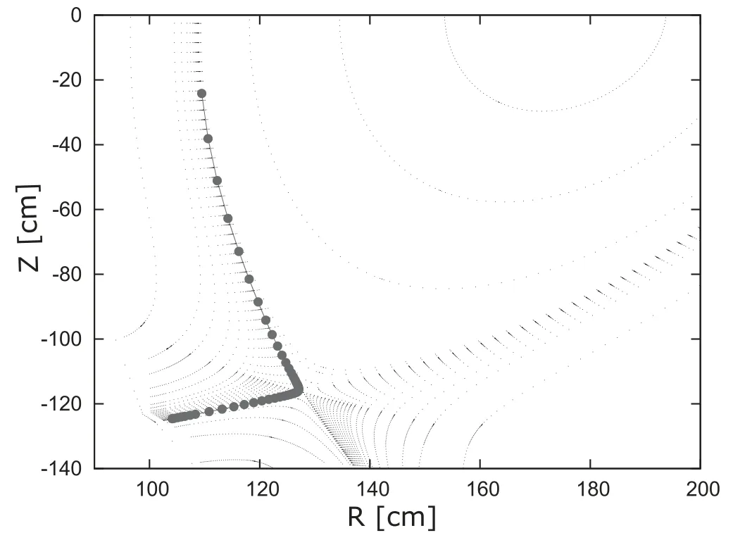
Figure 1.2D representation of the field line along which the plasma field values will be examined.

In this paper,errors are examined for the plasma field variables along an open field line close to the separatrix.The evaluation along the field line is cut off near the midplane.The red line in figure 1 shows the projection of the chosen field line on a poloidal surface,while the black dots indicate the grid points at this surface.The line is specifically chosen close to the separatrix as plasma profiles typically have relatively large gradients there and we,therefore,expect relatively large numerical errors.The error will be expressed as the L1-norm over the field values φnas follows:

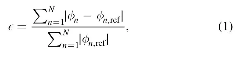
where the reference solutionφn,refis the most accurate,numerically obtained solution that is relevant for the error contribution(s)under investigation.This reference solution is,therefore,chosen differently depending on the examined error contribution.Numerical details are mentioned in later sections.The standard deviation of the iterations σ1,which is needed to evaluate the statistical error,is estimated using the sample standard deviation s:

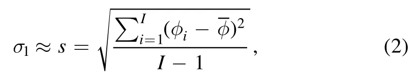
with I the number of iterations andthe average of φiover all iterations I after a statistically steady-state is reached (see next section).

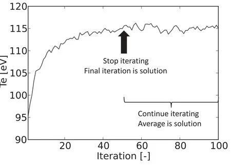
Figure 2.Evolution of the electron temperature Te in a cell close to the target in an EMC3-EIRENE simulation with two simulation approaches indicated (with and without post-processing averaging).

3.Simulation approach with post-processing averaging

In typical plasma edge simulations with EMC3-EIRENE,three modules are iteratively solved:energy (EMC3),streaming (EMC3) and neutrals (EIRENE).In the energy module,the ion-and electron energy equations are solved for the ion and electron temperature,Tiand Te.In the streaming module,the plasma continuity and momentum equations are solved for the plasma density n and the Mach number M.In EIRENE,neutral transport is simulated to estimate source terms for the plasma equations coming from plasma-neutral interactions.Starting from an initial condition,the modules are iteratively solved until the solution remains statistically stationary.To achieve convergence,it is often necessary to provide a relaxation (we take 0.6),which limits the change between iterations.

Convergence is usually measured by observing the development of the entire plasma during iterations.Suitable monitoring parameters are,for example,the total recycling flux and the average Te,Tiand neat the targets(e.g.weighted by the local plasma pressure).Strongly depending on the plasma regime under investigation and on the relaxation technique,the evolution could be so slow that the iteration process has to take longer than necessary in order to ensure a converged solution,in which the change of the monitoring parameters remains statistically stationary.So far,the final solution is taken from the last iteration.In this paper,we introduce a post-processing averaging method to improve the statistics.

With averaging,we continue iterating even after the solution has reached a statistically stationary regime.From this point,we start calculating the post-processing average,where we update its value on the fly,as explained in [10].This is graphically represented in figure 2,which shows the evolution of the electron temperature in a cell close to the target.We stress that the post-processing average does not interfere with the usual iteration process and is only used in post-processing.

Post-processing averaging is a well-known method to reduce the variance in iterative MC codes in many fields,like nuclear fission [11],statistical physics [12]and turbulent combustion[13].Within plasma edge simulations,it has been recently introduced in B2-EIRENE,where it led to an order of magnitude speed up in a partially detached ITER simulation[10].Also for SOLEDGE2D-EIRENE,it has been indicated that a similar gain can be achieved using averaging [14].Although,at first sight,it might seem to increase the computational effort,it is used in this work.Indeed,it can significantly speed up the simulation run time,as will be demonstrated in section 5.2.

4.Error reduction rates

The numerical errors consist of several contributions:the discretization error,the time integration error,the bias,and the statistical error.In this section,we examine how the error contributions behave as a function of the time step Δt,the number of MC particles per iteration P,and the number of iterations I.The analysis in this section excludes the effect of the grid resolution on the error (i.e.the discretization error),which will be discussed later in section 6.To simplify the analysis,we examine the accuracy of the energy module separately with a fixed background (density n,mach number M,sources)obtained from a fully coupled,converged EMC3-EIRENE simulation.The results of this analysis will be then applied to a fully coupled EMC3-EIRENE simulation in section 5.First,we discuss the time integration error,which is related to the time step Δt.Afterwards,the statistical error and the bias,which are present due to the finite number of MC particles,are elaborated.

4.1.Time integration error

MC particles in EMC3 are followed in small time steps Δt,with the corresponding random walk step determined bywith χ‖and χ⊥random unit vectors respectively parallel (1D) and perpendicular(2D)to the magnetic field,and with β‖,β⊥,α‖and α⊥respectively the diffusion (β) and advection (α)coefficients in the parallel(‖)and perpendicular(⊥)direction as determined by the model equations in Fokker–Planck form[5].Because perpendicular transport is much smaller,it is customary to choose a larger time step in the perpendicular direction while managing spatial accuracy.The field values n,M,Teand Tiare calculated from the particle trajectories using track length estimators in each plasma grid cell.These estimators accumulate contributions based on the time that a particle spent in the cell and the particle’s weight,which represents a fraction of the total source [5].

This random walk diffusion process is referred to as the Euler–Maruyama discretization,where particle trajectories displayconvergence in the strong sense and O(Δt)convergence in the weak sense[6].The tallies based on track length estimators are expected to exhibit a convergence order between these limits.The stochastic integration algorithm adopted in EMC3 has,therefore,an accuracy up to the first order.For the purpose of this work,it is sufficient to determine the order of convergence using only numerical experiments,without rigorous analysis.

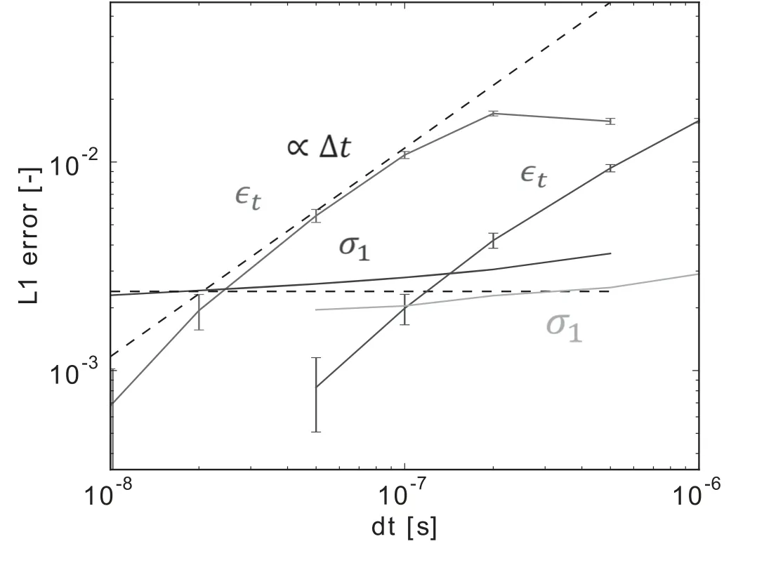
Figure 3.Time integration error ?t and standard deviation σ1 with a varying parallel (green,blue) and perpendicular (red,orange) time step Δt for the L1-norm of the electron temperature Te along the field line.

The integration errors of the stochastic process arise from non-uniform transport coefficients,including curvature-related terms in non-uniform magnetic fields,and from the boundary conditions,which reflect the finite size scale of an actual system.A natural way to evaluate this error would make use of the ratio of the jump step Δr to the variation lengths of the transport coefficients.In this paper,we choose to characterize the error as a function of the time step Δt,which is the control parameter of the displacement Δr.While this choice limits a general,physical interpretation of this error component,it is easy to use in practice.

To determine the order of convergence experimentally,the solutions from simulations (energy module only) with varying time step are analyzed.First,the parallel time step is changed,keeping the perpendicular one constant (Δt⊥=2 × 10-7s).Then,the perpendicular time step is varied,keeping the parallel time step constant (Δt‖=10-8s).From the electron temperature profile Tealong the selected field line(see section 2),the L1-errors ?tare calculated using the most accurate solution with respectively Δt‖=5 × 10-9s and Δt⊥=10-8s as the reference.As this reference point might be close to the set of points under investigation,care is taken to provide error bars that indicate the statistical uncertainty in the L1-norm coming from the statistical errors on both the investigated solution and the reference solution.All simulations are executed using P=105particles per iteration per processor on 20 processors.The solution is averaged over 100 statistically stationary iterations I.

For sufficiently small Δt,the observed order of convergence is approximately one,as can be seen from the green and red lines in figure 3 for respectively the parallel and perpendicular time step.Therefore,the time integration error(both parallel and perpendicular) can be approximated as

with At‖and⊥Atconstants,that can be calculated from the slopes in the figure.For large values of the parallel time step,the asymptotic regime is not reached yet.

Comparing the magnitude of the error with both time steps Δt‖(green) and Δt⊥(red),it is clear that the error related to the parallel time step is much larger for the same Δt:At‖≈ 10At⊥.This confirms that Δt⊥can be chosen an order of magnitude larger than Δt‖without becoming the dominant contribution and compromising accuracy.In the remainder of this paper,a perpendicular time step of 2 × 10-7s in the energy module is selected for convenience,while the parallel time step can be varied and will be indicated as Δt,without the subscript ‖.

The standard deviation σ1of the iterations is almost independent of the time step,as can be observed from the blue and orange lines in figure 3.This indicates that the magnitudes of the bias and the statistical error,which will be discussed next,are independent of the time step.

4.2.Bias and statistical error

The stochastic character of the MC particle trajectories in an iterative nonlinear MC code gives rise to a statistical error ?sand a so-called bias ?b[8].The bias is the deterministic component of the error,which exists due to nonlinearities,and decreases quickly with an increasing number of MC particles per iterationThis bias includes the so-called convergence error,which is present due to a remaining nonzero relative change[8].The statistical error has a probability distribution with mean 0 and a standard deviation σ.

The standard deviation σ characterizes the statistical error and is dependent on the number of MC particles per iteration P and the number of iterations I over which is averaged.The law of large numbers states that the standard deviation of an iteration scales with the inverse of the square root of the number of MC particles per iteration:

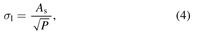
with Asa constant.When an average over several iterations I is taken,the statistical error decreases further

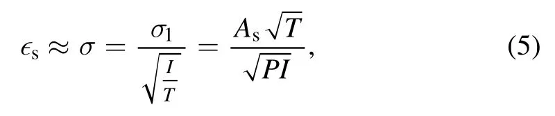
with T the correlation time,which is a measure for the dependency between consecutive iterations.It is interpreted as the number of iterations after which a new iteration is statistically independent.The constant Asis independent of P,I and Δt.

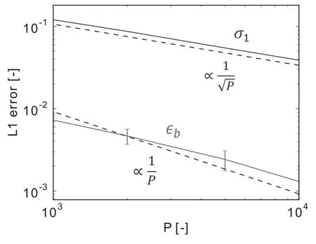
Figure 4.Bias ?b and standard deviation σ1 as a function of the number of MC particles per iteration P for the L1-norm of the electron temperature Te along the field line.

These errors are examined by analyzing the results of simulations obtained with several numbers of MC particles per iteration P,while keeping the time step constant(Δt=10-8s).In figure 4,we show the estimated values of standard deviations σ1(blue) and the bias ?b(green) for the L1-norm of the error on Tefor the chosen field line.The standard deviations σ1are estimated as sample standard deviations of the iterations.The bias is estimated from the averaged solutions (I=2 × 104) and using a reference solution with P=106(I=103).The error bars indicate the statistical uncertainty due to the remaining statistical errors on the averaged solutions.The correlation time T,which is relatively small (T ≈ 5),is estimated with the batching method(for more details,see[15,16]).Because of the minor importance of this factor and for clarity of notation in the analysis,the correlation time will be included in the constant for the statistical error:

It can be observed that the bias is relatively small compared to the standard deviation,even for a relatively small number of MC particles per iteration P.Therefore,the bias will not be of major importance in realistic simulations where a relatively high number of MC particles P is chosen.Even with small P,many iterations are required to reach a sufficiently small statistical error to evaluate the magnitude of the bias accurately.While the remaining statistical errors prevent the theoreticalreduction rate from appearing distinctly in this example,the order of magnitude can be observed clearly.Thereduction rate forσ1,on the other hand,is clearly confirmed.

Because the number of particles specified in the input file specifies a maximum weight of a particle relative to the source strength,the number of actually followed MC particles in an EMC3 iteration is not generally equal to the specified number.The MC algorithm ensures that particles will be transported from all the sources.Instead of following exactly P particles,EMC3 continues to launch new particles until all sources are accounted for.This guarantees a minimal accuracy in all parts of the domain.

In summary,the total error originating from the limited number of MC particles per iteration is expressed as

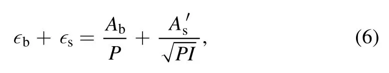
where Aband ＇Asare constants,which are independent of P,I,and Δt.

5.Accuracy in EMC3-EIRENE

In a fully coupled EMC3-EIRENE simulation,the energy,streaming and neutral modules are solved sequentially in each iteration.To estimate the accuracy,error contributions from each module need to be taken into account.First,we discuss the parameterized expression for the total error,excluding the discretization error,which is the topic of the next section.Then,after explaining the parameterized model for the CPUtime,the optimal parameters are determined to obtain a minimal error for a given CPU-time.

5.1.Error contributions

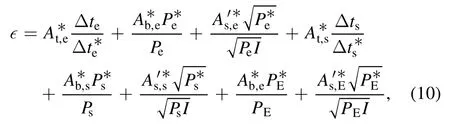
The total error on a quantity of interest needs to take into account the error contributions from each module.This is expressed by summing all the contributions of the energy ?ene,streaming ?strand neutral ?EIRmodule:

Like for the energy module,the error for the streaming module consists of a time integration error,a bias and a statistical error.In the neutral module (EIRENE),however,only a bias and a statistical error are present.No time integration error is present in EIRENE,because particle trajectories are followed kinetically from one interaction to the next one without an approximation in time.This results in the following equation:

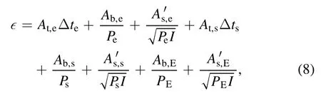
where the constants and parameters related to the different modules are indicated with the additional subscripts e(energy),s (streaming) and E (EIRENE).

As mentioned in section 4.2,the statistical error can be estimated by calculating the sample standard deviation σ1and making use of the law of large numbers.More details can be found in [9,16],where an identical approach is followed.

The constants for the deterministic errors can be estimated by comparing solutions with a different resolution.This method (often referred to as ‘Richardson extrapolation’)is typically used to determine the discretization error in finite volume codes [17],but can be applied to estimate any deterministic error with a consistent reduction rate.For parameter Y (which can be Δt or P for the errors ?tand ?brespectively),two solutions φYand φαYwith respectivelyresolution Y and αY are required,with α the scaling factor.Assumingwith pYa known order of convergence(pΔt=1andpP=-1),the error on solution φYis estimated as

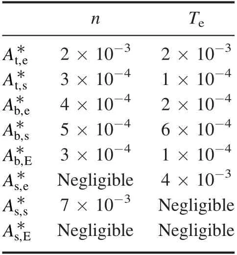
Table 1.Constants for the error contributions,according to equation (10).

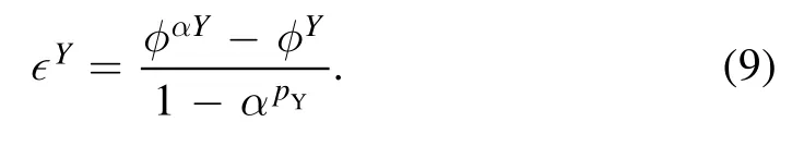
From this,the constant can be easily obtained asBecause the biases and time integration errors are relatively low,it is recommended to choose a lower resolutionφαYthan the standard choice φY.This will not only save CPU-time,but also likely provide a more reliable estimate [16].To obtain an accurate estimate,it is important to provoke the deterministic error that needs to be estimated,such that it is the dominating error in the differenceφαY-φY.Because equation(9)assumes that this difference is exclusively coming from ?Y,remaining statistical errors undermine its accuracy.Post-processing averaging can,therefore,improve the accuracy by reducing the unwanted statistical errors.Another potential source of inaccuracy is the assumption that the asymptotic regime is reached where the expected error reduction rate is valid.A too low resolution should,therefore,be avoided.Although it is difficult to achieve a reliable estimate using only two solutions,it can give a reasonable evaluation of the order of magnitude of the error.More details can be found in [9,16].

For the considered example,table 1 lists the approximate magnitude of the constants.Because these numbers represent the order of magnitude of the error rather than an accurate estimate,only one digit is given.For ease of interpretation,the typical parameter values are taken as a reference to scale the constants.This results in the following error equation:

? There is a clear difference in magnitude between the streaming and energy time integration error constants,andAt,e*,with the latter being an order of magnitude higher.This suggest that Δtscan be chosen higher than Δtewithout compromising accuracy,thereby consuming

less CPU-time in the streaming module.

? The several constants for the bias,andare of the same order of magnitude.Since also the relevant statistical errors (for the error on n andfor the error on Te) have a similar order of magnitude,choosing the number of MC particles approximately equal in each code module results in similar values for these errors.Whether this is the optimal choice of parameters also depends on the CPU-time required in each module,which will be discussed further in the next subsection.

? The constant for the statistical errorAs*is only relevant for the variables calculated in the module itself.The statistical error on the density,for example,is affected by the number of particles in the streaming module Ps,but not significantly by the number of MC particles in the energy module Peor in EIRENE PE.The latter (Peand PE) will only have an effect on the density error in an average sense,through the bias.

? The time integration error for the energy module and the statistical error are dominant and within ≈1% for the typical parameter choice in this example,excluding the discretization error.

The constants in table 1 will be used in the next section to analyze the optimal choice of numerical parameters to achieve faster and/or more accurate simulation results.We stress that these constants are estimated for this specific case (see section 2).Different values for the constants will be obtained for different conditions and plasma parameters.

5.2.Optimal parameters

Using parameterized expressions for the error and the CPUtime,the optimal choice of the numerical parameters(Δte,Δts,Pe,Ps,PE,I) can be determined to achieve a minimal error in a specified CPU-time.Before examining the optimal parameters,the model for the CPU-time is shortly discussed.

While the CPU-time required for each module scales linearly with the number of MC particles P and the number of iterations I,the dependency on the time step is less clear.In the considered practical range for the time steps,we fit a function of the form Δa tb,with a and b the fitted constants,to the measured CPU-times for several time steps in each EMC3 module.The red and blue lines in figure 5 show the measured CPU-times (full lines) and the best fit (dashed lines) for respectively the energy and streaming module.Since EIRENE is independent of the time step,its CPU-time is constant w.r.t.the time step(bE=0).Moreover,its value is relatively small,as can be observed by comparing the green line(EIRENE)in figure 5 to the red (energy) and blue (streaming) lines for the usual time step Δt ≈ 5 × 10-8s.These CPU-times are calculated as an average of the measured CPU-times for several iterations withP*=105on one processor.

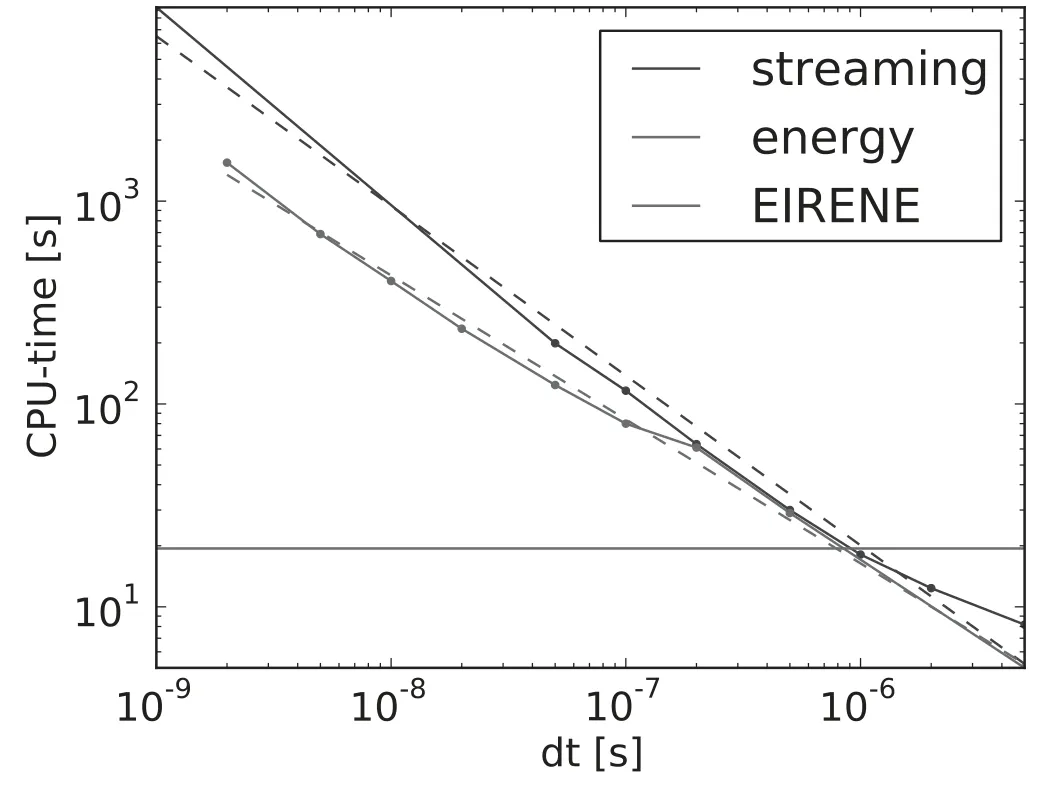
Figure 5.Measured CPU-times (full) and their fits (dashed) as a function of the time step Δt for each module for=P 105* on 1 processor.

The resulting parameterized expression for the CPU-time is the sum of the contributions of the energy,streaming and neutral modules:

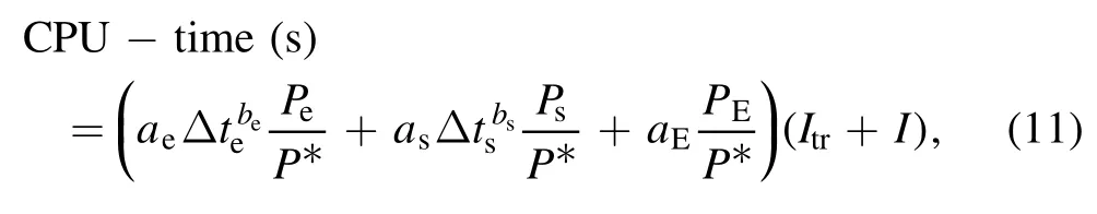
with Itrand I respectively the number of unsteady iterations in the transient,which have to be discarded,and the number of statistically stationary iterations,which contribute to the averaged solution.To take into account multiple parallel processors(20 here),it is sufficient for the purpose of this text to obtain the wall clock time by simply dividing the CPUtime by the number of processors,neglecting the overhead time.For this analysis,the following values have been used:ae=0.001,be=- 0 .7,as=0.000 2,bs=- 0 .8,aE=20.

Using optimized parameters,a specified numerical error can be obtained more than twice as fast than with the initial,non-optimal parameter choice.Alternatively,for the same amount of computational time,approximately twice as accurate results can be reached with optimized parameters than with the non-optimal approach.This is illustrated in figure 6,where the minimal errors that can be reached with optimized parameters (black) are compared to the error obtained with the non-optimal parameter choice (red,Δte=Δts=5 × 10-8s,I=1,Pe=Ps=PE).The selection of the optimal parameter choice is achieved by evaluating the total error for many parameter combinations in a large range and finally choosing the combination of parameters that provides the minimal error.Parameter scans have been performed over the six free numerical parameters:Δte,Δts,I,Pe,Ps,PE.For this optimization,we use the constants for the error on ni(see table 1,whereAs,eis substituted by its value for the error on Tein equation(10).Since all other constants (At,Ab) are of the same order of magnitude for n and Te,the error will be similar for both the energy and streaming variables,and large statistical errors on the temperature are avoided.The number of iterations in the transient and the correlation time are respectively Itr=50 and T=5.

Figure 6.Minimal error that can be obtained within a specified computational time for the non-optimal(red)and the optimal(black)choice of parameters.

To highlight the main differences between the non-optimal and the optimal approach,we discuss the minimal error that can be reached in 105s (≈1.2 d).By optimizing the numerical parameters,the total error is reduced by ≈50%.Details from all error contributions and the distribution of the CPU-time over the modules are illustrated in figure 7.Two aspects,which are discussed next,lead to the increased accuracy:the introduction of post-processing averaging which allows a lower choice of P,and the optimally chosen time steps.We stress that the simulation with the optimal parameter choice provides the solution in the same amount of computational time as the simulation with the original parameter choice.

Thanks to post-processing averaging,the total statistical error?s,e+?s,shas decreased by almost 50%,while the sum of the biases remains below 20% of the total error.To decrease the statistical error,both the number of MC particles per iteration P and the number of iterations I can be increased.With a lower choice of P(while keeping the time ∝P(Itr+I)constant),the time for the transient decreases,thus a higher share of the time contributes to the solution.Because the bias increases with a decrease in P,the optimal choice of P and I is a compromise between the statistical error and the bias.This optimum is typically wide and,thus,a large range of choices of P and I will lead to an increased accuracy [18,19].In this example(see figure 7),the number of iterations in the average was increased from 1 to 70,while the number of MC particles per iteration was decreased from 5 × 105in each code module to 3×105in EIRENE and the EMC3 streaming module,and 105in the EMC3 energy module.

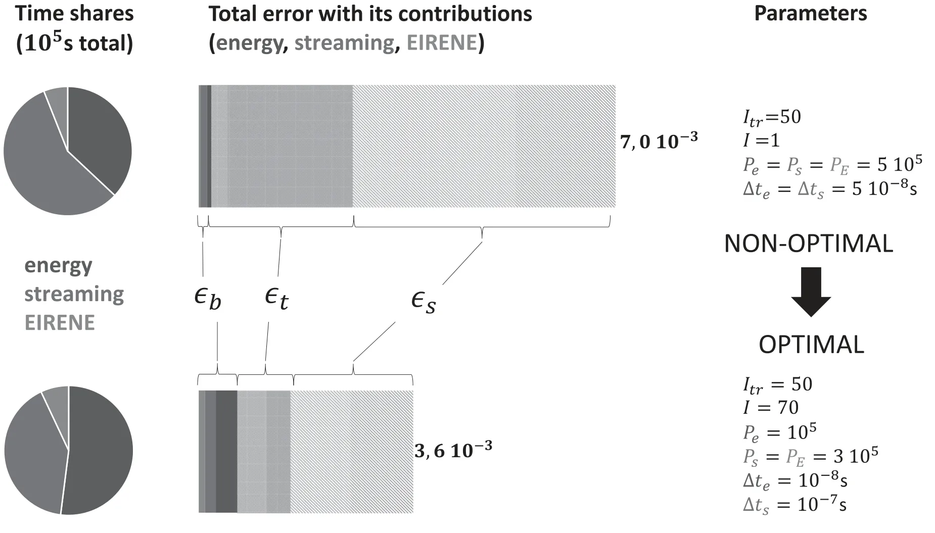
Figure 7.Shares of the computational time for the modules(left),magnitude of the error contributions(middle),and parameter choice(right)for the usual (top) and optimal (bottom) selection of numerical parameters for a wall clock time of approximately 105 s (≈1.2 d).

The total time integration error?t,e+?t,shas decreased drastically by exploiting the magnitude difference for the time integration error constants in the energy and streaming module.Time is saved by increasing the streaming time step Δtsfrom 5 × 10-8to 10-7s,with only a slight increase in?t,s.This time is now used in the energy module,where a smaller time step Δte(10-8s instead of 5×10-8s) significantly reduces the time integration error?t,e.The magnitude difference betweenAt,eandAt,sis present because the parallel viscosity term in the momentum equation is neglected in this example.The parallel transport of the MC particles is,therefore,deterministic,such that the parallel time step limit is determined by the cross-field transport.

We note that the computational time required for EIRENE is relatively small in this low recycling case.With larger neutral densities in high recycling or detachment regimes,we expect this share to increase.

While different optimal parameters will be obtained for different case studies,we illustrated that the computational performance of EMC3-EIRENE simulations can be substantially improved by choosing the numerical control parameters appropriately.Knowledge of the numerical error contributions is,therefore,not only necessary to assess the numerical quality of the solution,but can also be used to optimize the code performance.We specifically point out the benefit of using post-processing averaging to increase the computational efficiency of EMC3-EIRENE simulations.The decrease in statistical error by taking an average over subsequent iterations enables the use of a smaller number of MC particles per iteration P.Since the bias is typically very small for a realistic choice of P,the accuracy remains high even with a smaller-than-usual P.

6.Effect of grid resolution

Additional to the time integration errors,bias and statistical error,the limited grid resolution gives rise to a discretization error.First,the magnitude of this error component is discussed by comparing simulations on three successively higher grid resolutions.Afterwards,it is explained how this error affects the optimal parameter choice.

6.1.Discretization error

The approximations due to the finite number of grid cells give rise to a so-called discretization error.Within each grid cell,the value of the scored variables is assumed to be constant.Moreover,during particle trajectories,transport coefficients and source terms are calculated based on the background densities,velocities and temperatures obtained in the previous iteration.

To examine the effect of grid resolution on the accuracy of the solution,simulations have been performed on three successively finer grid sizes.Two finer grids have been constructed with a two and four times higher resolution in each dimension compared to the original grid.Each grid is constructed separately such that field alignment is ensured.In practice,the grid cells of the original,low resolution grid are approximately split in 8 and 64.The runs have been performed withΔte=0.2 Δts=10-8s,andPe=Ps=0.5PE=105on 20 processors.

The solution significantly changes with grid resolution,as can be seen from figure 8,where respectively the density(left) and electron temperature (right) profiles along the selected field line are shown for the low(red),medium(blue)and high (black) resolution grid.Clearly,the density decreases and the electron temperature increases with higher resolution.Differences between the low and high resolution solutions are of the order of magnitude 10%–15%.

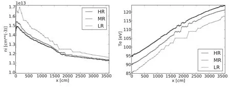
Figure 8.Density (left) and electron temperature (right) profile for three successively finer grid resolutions for the chosen field line.

In an MC code,second order convergence with grid resolution is expected (pX=-2),because the variables are approximated as piece-wise linear profiles in the particle tracking algorithm [8].The order of convergence pXis estimated using the following equation [17]:

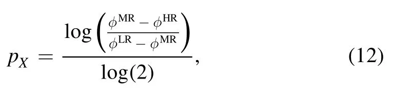
whereφLR,φMRandφHRare the solutions on the low,medium and high resolution grid,respectively.We evaluate pXat each location along the profile on the low resolution grid,which results in an average of pX=-1.9 for the density and pX=-0.50 for the electron temperature.The predicted order of convergence is thus retrieved for the density,but not for the electron temperature.We anticipate that the asymptotic regime is not yet reached for these relatively low resolution grids and we expect it to appear for higher resolutions.

The discretization error on the original low resolution grid is calculated to be 8% and 16% for the density and electron temperature respectively.This L1-error is calculated with a reference solution extrapolated from the medium and high resolution grid,assuming second order convergence.Comparing these values to the errors in table 1,we conclude that the discretization error is the dominant error contribution for the usual parameter choice.For the medium and high resolution grid,the discretization errors are estimated to be between respectively 5%–10% and 2%–5%.

The dominant discretization error demonstrates the need for a good grid resolution.Globally refining the grid,as done in this paper,is easy,but not optimal in practice.Indeed the computational time as well as the memory requirements increase considerably with a higher number of grid cells.The solution is most sensitive to the discretization in regions with large gradients and thus strong variations in the parameters.Optimized grids can exploit this by increasing the resolution only in these regions of the domain,which can be identified by comparing the physical length scales to the cell width.This example showed very large variations in the density and Mach number in the first cells next to the target.It is,therefore,expected that the numerical accuracy can largely benefit from an increased resolution near the target.

6.2.Optimal parameters

Since the discretization is dominant,we expect a large influence of the grid resolution on the optimal parameter choice.In this section,we include grid dependency in the equations for the error and the computational time and discuss its influence on the optimal parameters.

Apart from adding the discretization error to equation(8),the grid dependency of the other error contributions needs to be taken into account.Because grid cells are smaller,more MC particles will have to be followed to keep the same accuracy.The variance,therefore,increases with higher grid resolution.The following scaling has been approximately observedσ12∝X1.4,where X is the refinement in each direction (respectively 1,2 and 4 for the low,medium and high resolution grid).This is also the expected scaling for the bias.Concerning the time integration error,it has been verified that its magnitude does not significantly change with grid size.This results in the following parameterized equation for the total numerical error:

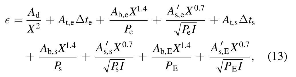
with Ad=0.08 and the other constants taken consistent with table 1.

For the computational time,equation(11)is used,where different constantsae,be,as,bs,aEare calculated for each grid separately.Estimates for these constants are obtained using runs with two different values for Δteand Δtswith P=105particles per processor on 20 parallel processors.This resulted in the following values:ae=1.4,be=-0.3,as=0.01,bs=-0.6 and aE=34 for the low resolution grid;ae=7,be=- 0.2,as=0.03,bs=-0.5and aE=40 for the medium resolution grid;ae=0.5,be=-0.4,as=50,bs=-0.16 and aE=80 for the high resolution grid.Although these estimates are rather rough because of the limited number of simulations,they give a sufficiently good representation of the computational times for the purpose of this text.

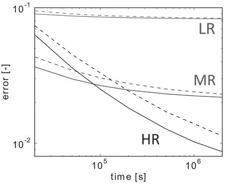
Figure 9.Minimal error,including the discretization error,that can be obtained within a specified computational time for the low (red),medium(blue)and high(black)resolution grid.The full and dashed lines represent the results with and without post-processing averaging,respectively.

A high grid resolution is required to achieve a small total error,as can be seen from figure 9,where the minimal error is shown as a function of the wall clock time on the low (red),medium(blue)and high(black)resolution grid.Averaging is the best choice in all cases,as can be seen from the difference between the full and dashed lines,which indicate respectively the results with and without averaging.It is clear that the error with the low resolution grid cannot decrease with time because the discretization error is dominant.Even for very small computational times,a higher accuracy can be obtained with the medium grid.With more time available (from ≈9×105s ≈1 d),the highest accuracy is obtained with the high resolution grid.The horizontal difference between the dashed(without averaging)and full (with averaging) lines indicates again a speed up of approximately factor 2.This speed up is thanks to the decrease of the statistical error with averaging.Of course,the advantages of averaging increase when the statistical error is dominant.

We conclude that the chosen grid resolution has a large influence on the numerical accuracy of the solution.For this example,even with a limited amount of computational time,the numerical error can be reduced from ≈8% to ≈3% by choosing a twice as high resolution in each direction than usual.This highlights the value of constructing more optimal grids for EMC3-EIRENE simulations.

7.Conclusion

In this paper,we demonstrated a framework to evaluate numerical accuracy and convergence in EMC3-EIRENE simulations.We also provided a first evaluation of the numerical accuracy with EMC3-EIRENE for the simulation of an axisymmetric DIII-D divertor edge plasma.This comprises the evaluation of all error contributions,originating from approximations due to the chosen time steps,the number of MC particles,the number of iterations and the grid resolution.Using parameterized expressions for the error and the computational time,we calculated the optimal numerical parameters to achieve a minimal error for a specified computational time.In this analysis,we made use of post-processing averaging for variance reduction,which significantly speeds up the simulations as results could be obtained approximately twice as fast for the same accuracy.Furthermore,we demonstrated that the discretization error,originating from the limited grid resolution,is the dominant error contribution with a magnitude of 10%–15%for the parameter choice as was originally used in this case.

With this analysis,we illustrated that simulations with EMC3-EIRENE can become significantly more efficient by applying post-processing averaging and choosing more adequate numerical parameters.We also demonstrated the substantial influence of the numerical grid on the accuracy,which stresses the importance of a good mesh construction and optimization.

Acknowledgments

The work of K Ghoos was sponsored by Flanders Innovation and Entrepreneurship (IWT.141064) and a travel grant(V4.128.18N) from Research Foundation—Flanders (FWO).Parts of the work are supported by the Research Foundation Flanders (FWO) under project grant G078316N.The computational resources and services used in this work were provided by the VSC (Flemish Supercomputer Center),funded by the Research Foundation—Flanders (FWO) and the Flemish Government—department EWI.