Stabilized seventh-order dissipative compact scheme for two-dimensional Euler equations?

Jia-Xian Qin(秦嘉賢), Ya-Ming Chen(陳亞銘),and Xiao-Gang Deng(鄧小剛)

College of Aerospace Science and Engineering,National University of Defense Technology,Changsha 410073,China

Keywords:compact scheme,time stability,simultaneous approximation term,interface treatment

1.Introduction

High-order finite difference methods are well suited for simulations of complex physics as they admit high resolution properties and save large amount of computational resources.Typical examples can be found in fluid dynamics.[1,2]Although the derivation of high-order finite difference schemes in the interior of the computational domain is quite straightforward,boundary closures often need special investigation[3–5]to avoid accuracy and stability issues.However,it is not an easy task to construct suitable high-order boundary closures to ensure stability.[3]

In our previous work,[6]we showed that a globally seventh-order scheme is not time stable when boundary conditions are imposed directly with the traditional injection method.To rectify this issue,we employed simultaneous approximation terms(SATs)[7]to impose boundary conditions weakly for a dissipative compact finite difference scheme,resulting in a time stable method with global accuracy of the seventh order.The method was demonstrated to be effective for solving one-dimensional(1D)problems,including linear advection equations and Euler equations.The aim of this paper is to extend the algorithm to solve two-dimensional(2D)Euler equations.

To this end,we need to make some modifications to the scheme since SATs involve some subtle issues in the 2D case.As will be seen in Section 2,around each corner of the 2D computational domain,there exists a small region where the boundary schemes involve boundary values from two different directions,which is different from the 1D case.Therefore,it necessitates to specially discuss the SATs in these regions to ensure stability.

We consider in Section 3 the implementation of the scheme for multi-block problems. In realistic computations the whole computational domain is usually divided into several subdomains with different grid finess to save computational resource considerably(compared with global refinement). For multi-block problems,some interface treatment techniques have to be used.[8–11]Here,the implementation of SATs provides a convenient interface treatment method,[12–14]which has been applied successfully to solve various problems by the summation-by-parts(SBP)community.[15–17]

Since curvilinear grids are often used in practice,we also discuss in Section 4 the implementation of the scheme to this kind of problems by focussing on two relevant examples.The SATs are still used in this case to ensure stability.Finally,conclusions are drawn in Section 5.

2.Extension to the 2D case

Consider the following two-dimensional Euler equations

where U=[ρ,ρu,ρv,E]Tis the conservative variable,F=[ρu,ρu2+p,ρuv,(E+p)u]Tand G=[ρv,ρuv,ρv2+p,(E+p)v]Tare the fluxes in different directions.Here the total energy is set to be E=ρ(u2+v2)/2+p/(γ ?1)with γ=1.4 for air.

2.1.Numerical scheme

To extend the seventh-order scheme considered in Ref.[6](some details can also be found in Appendix A)to solve Eq.(1),it necessitates to consider its quasi-linear form[18]

where the Jacobian matrices

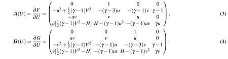
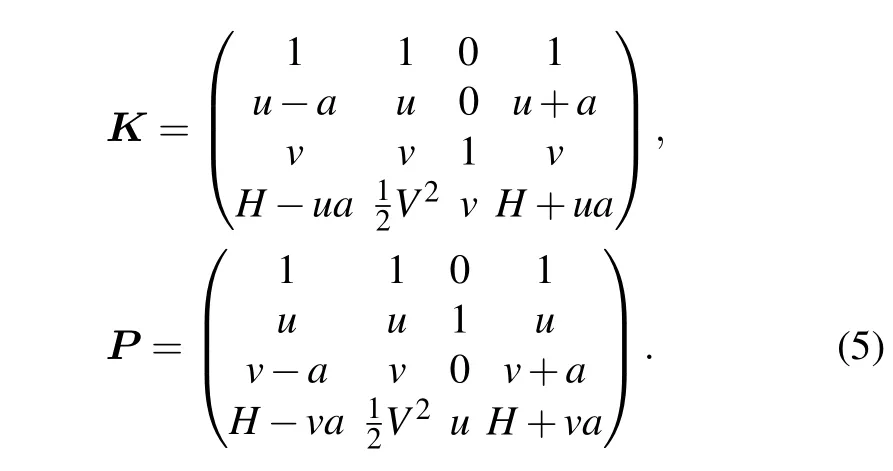
Here V2=u2+v2,and H=V2/2+γ p/(γ ?1)ρ is the specific enthalpy. In addition,the Jacobian matrices can be diagonalized as=diag{u ?a,u,u,u+a}and=diag{v ?a,v,v,v+a},whererepresents the sound speed,andread explicitly as

For a computational domain(x,y)∈[xw,xe]×[ys,yn],we denote the discrete coordinates by xi=xw+(i ?1)hxwith 1 ≤i ≤N and yj=ys+(j ?1)hywith 1 ≤j ≤M,where hx=(xe?xw)/(N ?1)and hy=(yn?ys)/(M?1)are the spacial steps in different directions.Let Ui,jand(Fx)i,jbe the approximations to U(xi,yj)and F(U(xi,yj))x,respectively,and similar notations for other fluxes and matrices.Then the interior semi-discrete scheme for Eq.(1)can be written as

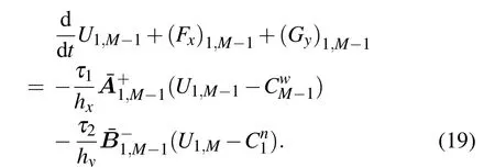
where the expressions for(Fx)i,jand(Gy)i,jare presented in Appendix A(see also Ref.[6]). For other points near boundaries,boundary values are involved,which are imposed weakly by using SATs.By introducing the notation

the approximations at the four corner regions read

For other points,the following semi-discrete approximations are used:

Here τk(1 ≤k ≤4)are penalty coefficients that can be tuned to stabilize the scheme,andstand for the well-posed west,east,south,and north boundary conditions,respectively. In addition,withwhere the notationrepresents the frozen value ofat the last time step.Similar notations also apply for.It is observed that the added SATs Si,jin Eqs.(7)–(14)vanish when the exact solution is switched into the scheme,meaning that the implementation of SAT method does not contribute to the truncation error and thus does not affect the convergence rate of the original scheme.

Intuitively,one may simply choose the penalty coefficients to be same values as the one-dimensional case,i.e.,τ1=τ2=τ3=τ4=5.[6]To test this choice,we take as an example the vortex model from Ref.[19],whose solution is given by

where f(x,y,t)=1 ?[(x ?x0?Ma∞t)2+(y ?y0)2]. Here the parameters(x0,y0)=(5,0),Ma∞=0.5,ε=1.0,and γ=1.4 are used. The computational domain is set to be(x,y)∈[0,10]×[?5,5]and the time step ?t=0.1hxhyis chosen to implement a traditional fourth-order Runge–Kutta scheme.If not stated otherwise,this time scheme will be used for other numerical examples presented in this paper.For simplicity,exact solution values are adopted at the boundaries.One can observe from Fig.1 that at t=4.2 the density solution near the right corners starts to deteriorate,while at t=6.3 the vortex is almost broken.This phenomenon indicates that some modifications for the scheme should be made to dissolve the non-physical error emerging from the corner regions,where the SATs from two boundaries overlap;see Fig.2(a).

Fig.1. Density contours of the vortex obtained by the scheme of Eqs.(6)–(14)with penalty coefficients τ1=τ2=τ3=τ4=5. Here N×M=41×81,the time step ?t=0.1hx1hy1 is chosen to implement the fourth-order Runge–Kutta scheme.(a)At the moment t=4.2.(b)At the moment t=6.3.

To show how to improve the scheme,we take as an example the solution point(x1,yM?1)at the west–north corner;see Fig.2(b). The semi-discrete approximation(9)at this point reads

Here the first penalty term imposes weakly the west boundary condition,whereas the second one imposes the north boundary condition.It is noted that the solution point(x1,yM?1)resides on the west boundary,which means that the second penalty term is not so important here.In this regard,we adjust the coefficient of the first penalty coefficient τ1to weaken the effect of the second one,while other coefficients remain unchanged.The same reasoning applies for other similar points. In this paper,we choose the penalty coefficients to be

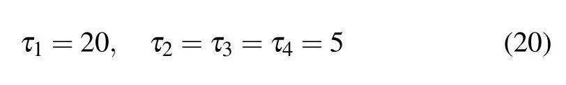
for the scheme of Eqs.(6)–(14),although the choice may be optimized further.

Fig.2.(a)Illustration of the computational domain.(b)The north–west corner area,where the solution points are affected by SATs from both boundaries.

2.2.Numerical example

Using the scheme of Eqs.(6)–(14)with the penalty coefficients(20),we recalculate the vortex solution of Eqs.(15)–(18).The new numerical results are presented in Fig.3,showing good preservation of the vortex.For accuracy test,we introduce the following L∞norm and L2norm:

The convergence rate is measured by

where e1and e2are the corresponding errors for different numbers of grid cells N1and N2,respectively.The results shown in Table 1 indicate that the expected seventh-order convergence rate is achieved approximately.

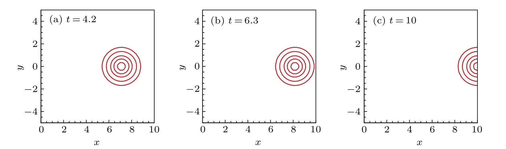
Fig.3.Density contours obtained by the scheme of Eqs.(6)–(14)with the penalty coefficients(20)on a 41×81 grid.Here the time step?t=0.1hx1hy1 is chosen to implement the fourth-order Runge–Kutta scheme.(a)At the moment t=4.2.(b)At the moment t=6.3.(c)At the moment t=10.

Table 1. Numerical test for the vortex solution of Eqs.(15)–(18)at t=10. Here the time step ?t=0.1hxhy is chosen to implement the fourth-order Runge–Kutta scheme.

3.Multi-block problems

In this section we intend to show that the developed scheme with SATs is well suited for multi-block problems,which are often used for complex configurations.

3.1.Interface treatment

For simplicity,the computational domain[xw,xe]×[ys,yn]is only divided into two subdomains with an interface situated at xk=(xe?xw)/2;see Fig.4. Denote the conservative variables in the left and right subdomains by Ui,jwith 1 ≤i ≤N1,1 ≤j ≤M and Vi,jwith 1 ≤i ≤N2,1 ≤j ≤M,respectively.In addition,assume that V1,jare the east boundary values for the left subdomain,and UN1,jare the west boundary values for the right.Then the problem can be solved by using the scheme of Eqs.(6)–(14)separately for each subdomain.

Fig.4.Density contours of the vortex of Eqs.(15)–(18)on the grid consists of two subdomains with 41×21 and 21×21 points. Here the time step ?t=0.1hx1hy1 is chosen to implement the fourth-order Runge–Kutta scheme.(a)At the moment t=0.(b)At the moment t=10.

To verify the scheme,we calculate the vortex convection problem of Eqs.(15)–(18)on the computational domain(x,y)∈[2.5,12.5]×[?2.5,2.5]with the split line x=7.5.The grid ratio is set to be 2:1 in the x direction.Figure 4 depicts that the vortex propagates successfully through the interface.One can also see from Table 2 that the convergence rates in both the two subdomains are well preserved.

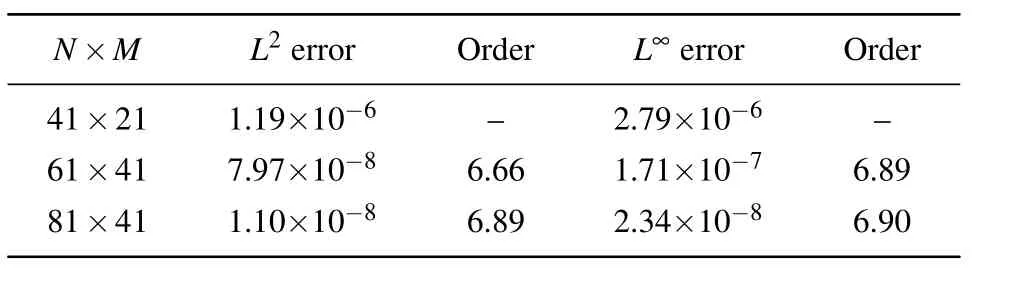
Table 2. Numerical test for the vortex solution of Eqs.(15)–(18)on two different subdomains with the grid ratio 2:1. Here the time step ?t=hx1hy1 is chosen to implement the fourth-order Runge–Kutta scheme.

3.2.Junction point

Next we demonstrate that by exchanging information through penalty terms,the interface technique can naturally handle grid partition with junction points. This time we divide the computational domain into four subdomains with two interfaces situated at xk=(xe?xw)/2 and yl=(yn?ys)/2,respectively.Here we still apply directly the scheme of Eqs.(6)–(14)to each subdomain with the boundary values at interfaces setting to be those of corresponding adjacent points;see Fig.5.

Fig.5.Illustration of information permutation at the junction point.

Fig.6.Density contours on the grid consists of four subdomains with 41×41(U),41×21(V),21×41(W),and 21×21(Z)points.Here the time step ?t=0.1hx1hy1 is chosen to implement the fourth-order Runge–Kutta scheme.(a)At the moment t=0.(b)At the moment t=5.(c)At the moment t=10.(d)At the moment t=15.

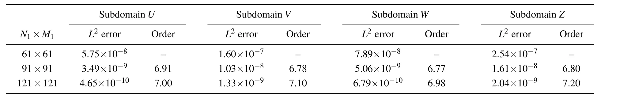
Table 3.Numerical test for the vortex solution of Eqs.(15)–(18)at time t=10 on four different subdomains with the grid ratio set to be the same as that presented in Fig.6.For brevity only the number of solution points in the subdomain U are presented in the table.Here the time step?t=0.1hx1hy1 is chosen to implement the fourth-order Runge–Kutta scheme.

Once again we consider the vortex convection problem of Eqs.(15)–(18)to verify the scheme.Here the computational domain(x,y)∈[2.5,12.5]×[?5,5]is chosen with interfaces situated at x=10 and y=0.It is observed from Fig.6 that the vortex propagates through the interfaces smoothly.In addition,the accuracy test presented in Table 3 shows that the scheme achieves its design order of accuracy approximately.

4.Discussions on curvilinear grids

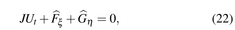
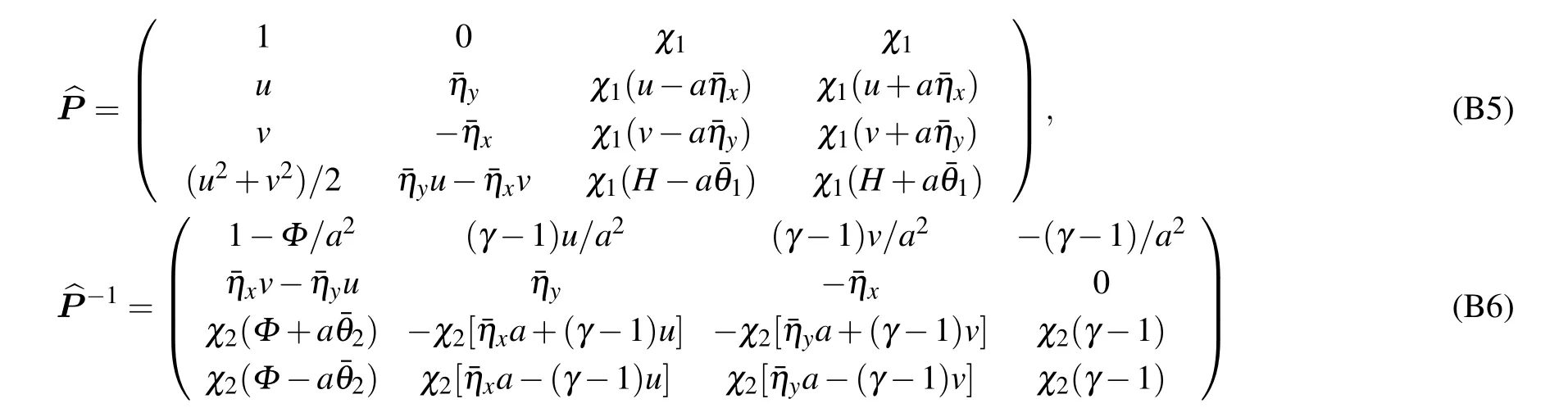
In this section,we study how to implement the numerical scheme for problems with curvilinear grids,which are often needed in practice for complex configurations. In this case,we need to consider the problem in the computational coordinates(ξ,η),where the Euler equations(1)read where the JacobianHere,we apply the difference scheme presented in Appendix A to calculate numerically the metrics xξ,xη,yξ,yη,and the Jacobian J.To ensure stability,it still necessitates to use SATs similarly to the case for Eq.(1)on Cartesian grids;see e.g.,Eq.(19).For convenience of the reader,some necessary formulae of the Jacobian matrices of the fluxesandare presented in Appendix B to implement the similar scheme as Eqs.(6)–(14).

4.1.Stationary model

The first example is a model governed by the following Euler equations with a source term

where the source term is determined analytically by S=Fx+Gyso that the problem admits the following stationary solution[20]

The numerical test for the stationary model of Eqs.(23)–(27)is shown in the following Table 4.

Table 4.Numerical test for the stationary model of Eqs.(23)–(27).Here the time step ?t=0.01hx is chosen to implement the implicit Euler scheme.

Fig.7.(a)Illustration of a 41×41 curvilinear grid.(b)Final density contour obtained on the 41×41 grid.

The curvilinear grid[21]considered here(see Fig.7(a))is generated from the standard computational domain(ξ,η)∈[0,1]×[0,1]by

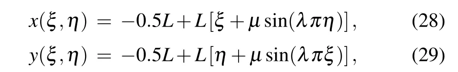
where the parametersμ=0.02,λ=6,and L=0.5 are chosen.The implicit Euler scheme is implemented for time-marching until the residue reaches machine zero(see Fig.7(b)for the final solution).

4.2.Nozzle flow

Consider a channel flow[22,23]governed by the Euler equations(1). The physical domain(Fig.8(a))is bounded between x=?0.75 and x=0.75 in the x direction,and is bounded by

in the y direction. The grid is produced analytically by the expressions

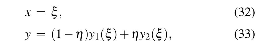
with ξ and η being partitioned equally.

The initial flow field is set to be the free stream with Ma∞=0.3,ρ∞=1,p∞=1,u∞=Ma∞·a∞,v∞=0,whererepresents the sound speed.The left boundary is set to be subsonic inflow while the right is subsonic outflow.Both the top and the bottom are set to be slip-wall boundary conditions.How to impose the slip-wall boundary condition weakly is explained in Appendix C.

Fig.8.A grid of the channel with 61×41 solution points and the corresponding numerical result of the density.(a)The 61×41 mesh.(b)Final flow field.

We run the calculation on a grid with 61×41 solution points until the residue reaches the machine zero. It can be observed from Fig.8(b)that the obtained density contour is smooth,showing the effectiveness of the scheme.Similar results can also be obtained on other grids with different finess.As the focus here is just to test whether the scheme is applicable for the case with curvilinear grids and wall boundary conditions,the convergence rate will not be discussed,which depends also on the smoothness of grids and the implementation of boundary conditions.

In addition,to compare the results obtained by the modified scheme and the scheme with the same penalty coefficients as Ref.[6],we show in Fig.9 the density contours and velocity vectors near the bump at t=0.054.It is observed that while the unmodified scheme starts to break up,the modified one still preserves well,demonstrating again that the modified coefficients are necessary to ensure stability.

Fig.9.Density solutions and velocity vectors near the bump obtained on the 61×41 grid at t=0.054.(a)The unmodified result.(b)The modified result.

5.Conclusion

In this paper,we generalized the globally seventh-order dissipative compact scheme with SATs[6]to the 2D Euler equations. The choice of penalty coefficients for SATs was reconsidered to stabilize the scheme. It was shown that the scheme with SATs is very convenient for dealing with multiblock problems with conformal grids.In addition,the implementation of the scheme for the case with curvilinear grids was also discussed,including the slip-wall boundary condition.Various numerical experiments were performed to verify the proposed scheme.The extension to Navier–Stokes equations may be considered in further work.

Appendix A:Spacial discretizations

Here we revisit briefly the spacial schemes presented in Ref.[6].For the one-dimensional conservation law

partition the computational domain[xl,xr]by using solution pointsand flux points xj+1/2=where N is the number of solution points,andis the spacial step.Let Ujandbe approximations to U(xj,t)and F(U(xj,t))x,respectively.Notations for other variables and matrices introduced in Section 2 are still adopted.The exact left and right boundary values are given by

Then the derivative of flux can be computed by the following formulae:for 5 ≤j ≤N ?4(i.e.,the interior points),

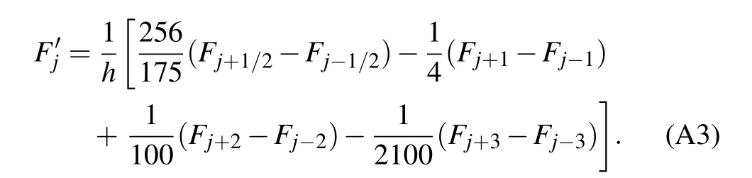
For near left boundary points we use the following difference schemes:

and the schemes for the right can be obtained by symmetry.

While the values Fjinvolved in the above difference scheme can be computed directly by Fj=F(Uj),the valuesare calculated by any approximate Riemann solver(in this paper Roe’s Riemann solver is adopted). Herestands for the left and the right values obtained by using the seventh-order dissipative compact interpolation scheme[1]: For the interior flux points ξj+1/2(3 ≤j ≤N ?3),

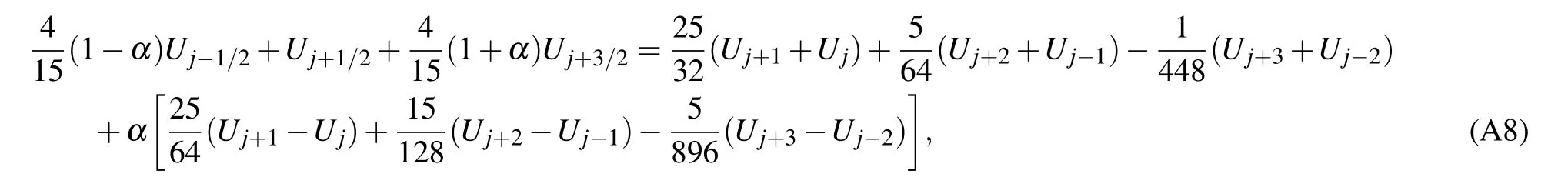
where the dissipation constant α=?0.3 is used for the left upwind interpolation,and by setting α=0.3 the interpolation becomes right upwind automatically. Due to the limitation of stencil length,the interpolations at near boundary flux points become

Appendix B:Jacobian matrices of fluxes in Eq.(22)

where J is defined in Eq.(22),.

Appendix C:Slip-wall boundary condition

Here we introduce for the two-dimensional Euler equations the slip-wall boundary condition imposed through SATs proposed in Ref.[24]. Consider a Cartesian grid and suppose that we are considering a point(1,j)situated on the wall boundary.Taking Eq.(11)as an example,i.e.,