Non-Stokes drag coefficient in single-particle electrophoresis:New insights on a classical problem

Mai-Jia Liao(廖麥嘉), Ming-Tzo Wei(魏名佐), Shi-Xin Xu(徐士鑫),H Daniel Ou-Yang(歐陽新喬), and Ping Sheng(沈平)

1Department of Physics,Hong Kong University of Science and Technology,Clear Water Bay,Kowloon,Hong Kong,China

2Department of Physics,Lehigh University,Bethlehem,PA,USA

3Department of Bioengineering,Lehigh University,Bethlehem,PA,USA

4Centre for Quantitative Analysis and Modelling(CQAM),The Fields Institute,Toronto,Ontario M5T 3J1,Canada

Keywords: electrophoresis,drag coefficient,vortices belt,charged colloidal particle

1. Introduction

When immersed in an electrolyte solution, a charged particle would be enveloped in an ionic cloud of screening counter-ions, denoted the Debye layer. Application of an external electric field to a suspension of such charged particles can result in the steady motion of the solid particulates.The physical picture underlying this phenomenon, known as electrophoresis,[1-5]dates back to Smoluchowski[6]in which the crucial element is the electroosmotic fluid flow in the Debye layer. Through clever mathematical manipulations,Smoluchowski has shown rigorously that electrophoretic mobility of the charged particle,μE,is directly proportional to the zeta potential ζ (which is directly related to the surface charge density)on the surface of the solid particle,i.e.,v∞=μEE∞,where E∞is the applied electric field,v∞is the electrophoretic velocity, and μE= -(ε/η)ζ, with η, ε being the solution viscosity and dielectric constant, respectively. The Smoluchowski relation is accurate in the limit of a ? λD,where λDis the Debye length and a the particle radius. A derivation of the Smoluchowski relation is given in Section S2 in Supplementary material.

There have been extensive theoretical[6-14]and experimental[15-20]studies of a charged particle under the simultaneous effect of an electric field E∞and a non-electric force Fext. In particular, the electrophoretic drag coefficient γEis of interest. This is because not only the Smoluchowski electrophoretic flow field(see Section S2 in Supplementary material) differs significantly from the Stokes flow field, but also the lack of an accurate flow field solution inside the Debye layer prevents an accurate account of the actual hydrodynamic drag force on the solid surface of the charged particle.A rough evaluation of drag force on the particle surface may be established through a simple scaling argument.[14,21]In the thin-Debye layer electrophoresis, the velocity gradient in the liquid is screened beyond the λDscale, thus the drag force is(4πa2)η/v∞. As a/1 in most cases, it follows that(=6πηa, the Stokes drag coefficient), with the ratioreaching as high as 100 to 200 in some cases.However,our accurate measurements of γE,described below,does not come anywhere close to such order of magnitude deviation from the Stokes drag. This large discrepency necessitates an understanding of the physical picture underlying the electrophoretic drag.

Based on the linearization of coupled electrohydrodynamic equations, plus the superposition of external nonelectric force Fextand the electrophoresis problem,[1,21]it is found that a charged particle behaves similarly in an electric field as in a hydrodynamic flow.[22]From force balance one obtains:where v denotes the solid particle velocity under the combined electric and non-electric (mechanical) forces. Equation (1)suggests that the mechanical force needed to stall an electrophoretic motion is a Stokes-like drag force.

In anticipation of subsequent developments,we make two remarks in relation to Eq.(1). The first is that equation(1)can be expressed in terms of two equations by the velocity decomposition v=v∞+Δv, where the first equation, v∞=μEE∞,is the definition of the electrophoretic velocity. The second equation is then Fext-γsΔv =0. Such a decomposition is useful in demonstrating that the electrophoretic drag coefficient γEis not necessarily identical to γS. This can be easily seen by multiplying the velocity equation on both sides by γE:FE=γEv∞=γEμEE∞=QeffE∞. Here γEis simply defined to be the coefficient of proportionality between velocity and hydrodynamic viscous force, in this case both resulting from an applied electric field,and Qeff=γEμEis introduced to distinguish it from the surface charge, since Qeffis known to be much smaller than the surface charge[14,16]and represents,in the context of force balance,the solid particle’s coupling to the applied electric field.

The second remark is related to our experimental approach of using an optical trap to hold a single charged particle in a harmonic potential and applying an AC electric field to induce periodic oscillations of the particle. The accurately measured quantities are then the amplitude of particle’s periodic motion and its phase difference with the applied AC electric field. Owing to the AC nature of the applied electric force,there are inevitably the in-phase and out-of-phase components of the force relative to the particle velocity. For Eq. (1), i.e.,Fext-γsΔv =0, the applied Fextis necessarily the in-phase component of the force, it describes that the force needed to alter, or stall, an intrinsic electrophoretic motion is Stokes by nature as argued by Long et al.[21]and thus,the equation itself has nothing to do with electrophoresis. Our simulation results(see below)supports the correctness of Long’s argument, but contradicts the non-Stokes prediction of the in-phase external force by Lizana et al.[14]We will show below in the subsequent section that in our experiment the optical trapping force is always out-of-phase relative to the phase of the velocity,whereas the applied electric force has both an in-phase component and an out-of-phase component.The in-phase component of the electric force drives the particle velocity and the out-ofphase component automatically counter-balances the out-ofphase optical trapping force. These facts account for our approach’s ability to measure the electrophoretic drag force and its drag coefficient.

The drag coefficient is always related to the hydrodynamic drag force exerted on a surface. As Smoluchowski has successfully linked μEto the surface zeta potential, and measured drag force is given byγEv∞=γEμEE∞=QeffE∞,achieving force balance between the electrical force and drag force at the solid surface(by equating Qeffto QS)would seem to be the most convenient choice. However, the fact that Qeffis known to be much smaller than QS,[14,16]which is also confirmed by our measurements as seen below,indicates that there must be another surface,away from the solid surface,[23-26]on which the drag force and electrical force attain force balance.Two questions naturally arise: (i) How does such a surface emerge consistently from the relevant mathematical equations governing the electrophoresis, and (ii) Can one measure an electrophoretic drag coefficient γEthat is consistent with the theory prediction on such a surface?

To address these two questions, we set out to measure γEand Qeffdirectly by experiments, and to obtain mathematically accurate simulations of the electrophoretic flow field.From experimental measurements the mobility was obtained as μE= Qeff/γE. It is shown that while γE/γSvaries only from 1 to 3 over a range of salt concentrations,the magnitude of Qeffis smaller than that of QSby many orders of magnitude. The resulting μE, however, agrees well with the literature values on similar micro-spheres, as well as that obtained by DC measurements in our experiments.[26]To provide a microscopic explanation of our experimental data, we have carried out simulation of the electrophoresis effect by numerically solving the Poisson-Nernst-Planck (PNP) equations coupled with the Navier-Stokes(NS)equation, implemented with the appropriate boundary conditions. Using only the experimentally measured μEas input, the most significant outcome is that the measured γEand Qeffare obtained at a uniquely distinctive interface between the inner and outer flow fields that is at a distance a few λD’s away from the solid surface. While the electrophoretic flow in the outer flow region follows the scaling of the Smoluchowski solution,i.e.,r-3,our numerical solution reveals an inner flow field that is carried along by the solid particle, with a highly nonlinear electro-hydrodynamic flow behavior. The interface between the inner and outer flow fields acts as the reference surface, or slip surface/plane, at which both the magnitude and trend(e.g.,with respect to salt concentration)of the drag coefficient and effective charge can be accounted for,and from which the deviations can be further explored.

In what follows,we first present the experimental results,followed by simulations and discussion of the physical picture that emerges. We end by underscoring the closure between theory and experiment.

2. Materials and methods

An optical trap was effected by an IR (wavelength =1064 nm) laser coupled into an oil-immersion objective lens(100X, NA = 1.3, Olympus). A second IR laser beam(wavelength=980 nm),aligned and focused by the same objective lens to be par-focal with the trapping laser focus, was used for particle tracking. A schematic diagram of the measurement apparatus is shown in Fig.S1 in Supplementary ma-terial. Here, we use the optical trap both as a tool to control/monitor the position of the particle as well as a calibrated force sensor[27-29]with a stiffness constant ktrap= 17.9±0.1 pN/μm. Experimental details are given in Section S3 in Supplementary material.

Polystyrene(PS,Thermo Scientific,catalog#5153A)particles with a mean radius a=0.75μm were dispersed at volume fractions below 1×10-4in solutions of varying concentrations of potassium chloride electrolyte with a Debye length λDranging from 96 nm to 4.3 nm(KCl concentration 0.01 mM to 5 mM, κa(≡a/λD) ranging from 7.8 to 174). To reduce the effect of dissolution of CO2in DI water, all electrolytes were prepared with fresh DI water filtered with resin. The colloidal solutions were inserted in a glass chamber with vertical height ～200 μm. To avoid the effects of the Fax′en drag on the particle[30-32]and the flow due to any surface electroosmosis flow near the glass surface,[33]we kept the colloid sphere 8μm-15μm above the lower glass plate.

The electrophoretic chambers were fabricated by coating a glass microscope slide substrate with Sigmacote (Sigma-Aldrich),a solution of chlorinated organopolysiloxane in heptane that readily forms a covalent,microscopically thin film on glass, with a purpose to suppress surface charge and to minimize surface electroosmotic flow. Subsequently gold wires for applying the electric field were placed on the glass substrate with a separation of ～1 cm. An aqueous solution of dilute particles was then dipped onto the substrate,and a Sigmacotecoated cover-glass was used to seal the chamber with wax sealant. External electrical wires were welded with the gold wires. Electric field was measured by inserting a second pair of parallel gold wires, separated by 5 mm, into the sample to obtain the voltage drop between them. The optical path diagram is shown schematically in Fig.S1 in Supplementary material. The electrophoresis chamber containing the particles was mounted on an inverted microscope(Olympus IX81). To minimize the contribution to the optical trapping effect, the 980-nm tracking beam power was two orders of magnitude lower than that of the 1064-nm laser. Movements of the particle, tracked by the 980 nm laser beam, were detected by a quadrant photodiode (QPD, S7479, Hamamatsu). The voltage reading of the QPD was maintained to be within the linear range of the particle displacement from the trapping center.A lock-in amplifier (SR830, Stanford Research) was used to record the phase of particle motion relative to that of the sinusoidal voltage applied to PZT to form an oscillatory optical tweezers. The wide-field images of the particle were captured by a CCD camera for the purpose of optical alignment.

3. Experimental results

3.1. Optical trap and AC electric field

We apply an AC electric field(20 Hz-100 Hz)to a single spherical particle held by a calibrated optical trap as shown in Fig. 1(a). At such frequencies the period of the applied field was much smaller than the time required to screen the electrodes(＞1 s for a separation between the electrodes=1 cm),and much larger than the relaxation time of the electrical double layer[34](＜1μs).The relevant equation of motion is given by:

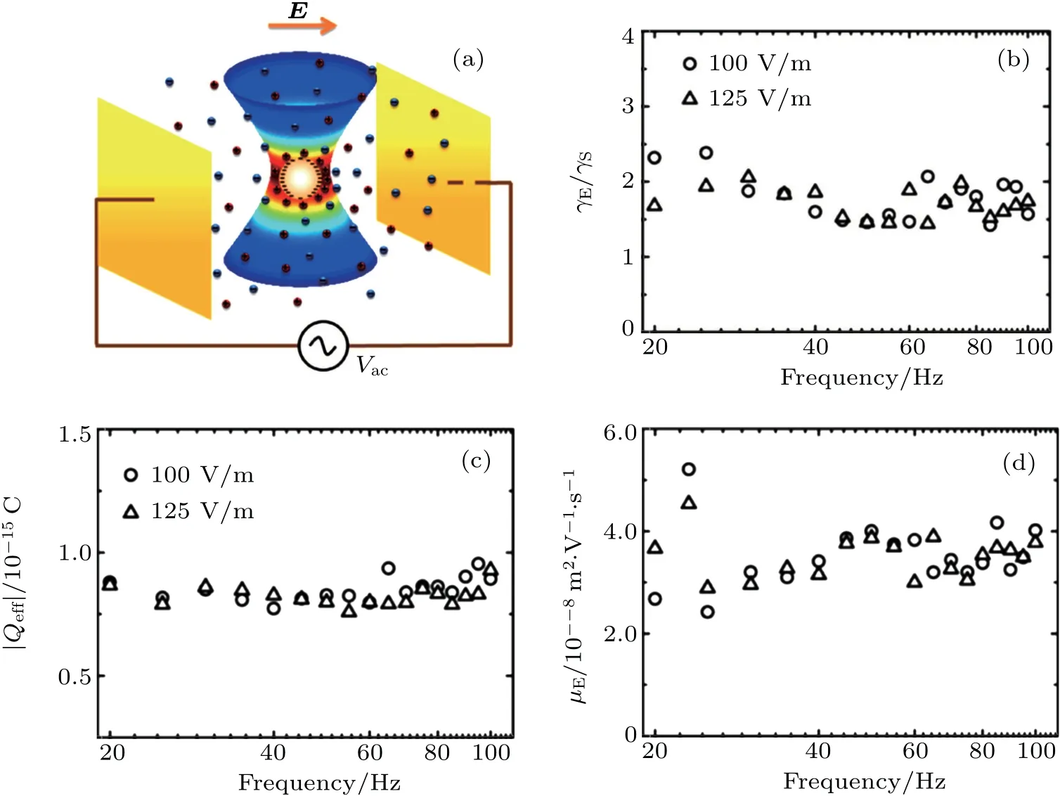
Fig.1. Electrophoretic measurements using the optical tweezers. (a)Schematic illustration of a charged colloidal particle held by an optical tweezer and driven by an oscillating electric field. The electric field direction is indicated for a particular instant of time. The measured γE/γS(b),magnitude of Qeff(c),andμE(d)plotted as a function of applied electric field frequency for a 0.75-μm radius polystyrene particle,held by a fixed optical trap in DI water(λD=96.1 nm)under two different electric field strengths. It is seen that all measured quantities are relatively independent of the frequency,indicating the quasi-static nature of the experiment.

Here, m is the mass of the particle, x is the displacement of the particle from the center of the harmonic optical trap, and γ is the drag coefficient. Here the drag coefficient is purposely written without a subscript, since in Eq. (2) there are two forces - optical trap force and electric force - acting on the particle and hence the specification of which drag coefficient applies would depend on the situation to be analyzed below. The Brownian noise term is excluded in the above equation because its contributions will be filtered out by the phase-sensitive, lock-in detection technique employed in our experiments. Here Qeffis the effective charge that provides particle’s electrical coupling to the applied electric field. It should be noted that the deformation of the counterion cloud is very small,so that the resulting electric“retardation”force can be neglected.[35]Our simulations,based on the full numerical solution of the relevant governing equations, have confirmed the negligible effect of retardation.

By approximating the left-hand side of Eq.(1)to be zero,which is accurate considering the fact that mω2is 5 orders of magnitude lower than ktrap,we have:

where E∞=E(0)∞exp(-iωt).We write the displacement of the electrophoretic particle as x(t)=D(ω)e-i[ωt-δ(ω)], with the displacement amplitude denoted by D(ω)and the phase δ(ω)defined relative to the applied AC electric field. In our experiments,the phase shift was measured with a lock-in amplifier with an accuracy of a couple of degrees. This is in contrast to the phase shift measurements in a previous paper[15]that has errors in the range of+/-11 degrees. Through the precise measurement of the phase shift, our method enabled the extract of drag coefficient value in an accurate and robust manner.

3.2. An analysis of the AC experimental approach

Substituting particle displacement expression for x(t)and the associated displacement velocity ˙x(t) back into Eq. (3),and taking the real part of every term,we get

Let us define a t0such that ωt0=δ(ω)+π/2, and let ωt =ω(t0+t′)=ωt0+ωt′. Equation (4) can be re-written in an illuminating form as

At t′=0,the left-hand side vanishes,i.e.,optical trap force is zero,and we only have the right-hand side,from which we obtain

We label the drag coefficient as γEbecause there is only the electric field force present in Eq.(6). Now let us expand

in Eq.(5). Then equation(5)can be re-organized in a physically clear manner as

In Eq.(7),the right-and left-hand sides represent the in-and out-of-phase components, respectively. There is no approximation made in Eq. (7), thus it has to be valid for all values of t′. The only way equation(7)can be true is that both sides must separately be zero, since the time variations on the two sides are orthogonal to each other.

Physically, equation (7) states that the electrical force comprises two components. One component,E(0)∞Qeffsinδ(ω)cos(ωt′),gives rise to the time-varying electrophoretic velocity ωD(ω)cos(ωt′)with a constant drag coefficient γE. The other component,E(0)∞Qeffcosδ(ω)sin(ωt′),counter-balances the optical trap force ktrapD(ω)sin(ωt′).This optical trap response force is noted to be out of phase with the electrophoretic velocity, in contrast to the external force in Long’s equation(Eq.(1)),which is in-phase with the electrophoretic velocity.

Equation(7)essentially expresses the fact that 0=0,from which we obtain two independent equations:

Equation(8b)is identical to Eq.(6). And if we divide Eq.(8b)by Eq. (8a), we obtain the consistency condition imposed by the force balance of the in- and out-of-phase components of the AC experiment:

Equation(8a)can be re-written for Qeffin terms of the physically measured quantities as

From Eqs.(9a)and(9b)the mobility is obtained as

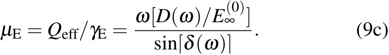
Not limited by the constraint imposed by typical DC measurements that any external non-electrical force would alter the intrinsic electrophoretic motion and yield a Stokes-like drag,the most essential point of the above analysis is that the external force imposed by the optical trap is always 90 degrees out of phase with the electrophoretic velocity. Through this feature of the AC electric field-driven particle in an optical harmonic trap,we can measure electrophoresis drag coefficient γEaccurately without the influences of an in-phase,non-electrical external force.

3.3. Measured drag coefficient, effective charge and mobility

Using the measured values D(ω)and δ(ω)in Eqs.9(a)and 9(b), respectively, we have evaluated γEand Qeff,which are plotted in Figs. 1(b) and 1(c) as a function of applied electric field frequency for a 0.75-μm radius polystyrene particle, held by a fixed optical trap in de-ionized (DI) water(λD= 96.1 nm) under two different electric field strengths.In Fig. 1(d) we show the measured values of μEplotted as a function of applied electric field frequency, also for two different electric field strengths. It is seen that the measured γE,Qeff,andμEwere relatively independent of the frequency and the field strength,indicating the quasi-static nature of our measurements, we take as measured values the averages over the measured frequency range.

It should be noted here that although the electrophoretic mobility determined from Eq. (9c) was determined from the AC measurements, we have also measured it using the traditional approach by using a DC field. Experimentally,this was done by turning off the optical trap and measuring the speed of the same particle in the presence of a DC electric field. The mobility determined by the AC measurements agreed with that by the DC measurements, as expected. It should be noted that the more precise phase shift values in our measurements clearly show the phoretic drag to be non-Stokes, while simultaneously the electrophoretic mobilities obtained by our AC and DC measurements agree within the experimental error. This is in contrast to the earlier experiment by Semenov et al.,[15]in which the phase shift measurement had a much larger error bar. Moreover, by assuming the drag coefficient to be Stokes,Semenov’s study yielded different mobilities between their AC and DC experiments.

In Fig. 2(a) the measured γE/γSis plotted as a function of κa with open symbols,where κ =1/λD. Non-Stokes drag coefficients values are clearly observed. As κa increases towards 110, however, γEgradually approaches γSwhich is in direct contrast to the 4πηa2/λDvalue of the scaling argument in the thin Debye layer limit.[14,21]

Fig.2.Measured drag coefficient and effective charge plotted as a function of salt concentration, expressed here as κa, where κ =1/λD. (a)Open symbols denote the values of measured γE/γS plotted as a function of κa. Here γS denotes the calculated Stokes drag coefficient,and γE is obtained by using measured δ in Eq.(9). Error bars on the open circles arise from the errors in amplitude and phase measurements. (b)Measured effective charge magnitude |Qeff| is plotted as a function of κa with open symbols. Filled symbols indicate the surface charge magnitude |QS| obtained from simulations with measured mobility μE as the only input from the experiment. Error bars are from the mobility measurements. All results are for PS spheres with a=0.75μm.

Values of the measured magnitude of the effective charge|Qeff| are plotted with open symbols as a function of ionic strength in Fig. 2(b). They are in the range of 1700 to 4800 electronic charges, which are one to two orders of magnitude smaller than the generally accepted values deduced from known PS surface charge density[26,36,37]that is in the range of ～-6×104e/μm2. For a 0.75-μm radius PS spheres, one obtains |QS|～1.9×105e, where e denotes the magnitude of the electronic charge. In Fig. 2(b), the magnitude of the surface charge|QS|obtained from our numerical simulations,ob-tained with the experimentally measured mobility values as inputs,are shown by solid symbols,these values are noted to be in the expected range of|QS|for PS surfaces, thus further confirming the huge differences with the magnitude of the effective charge. Also, as QSis always directly related to the mobility,the resulting zeta potential/mobility relation is compared to the literature in Section S5 in Supplementary material.Excellent agreement is obtained.

4. Simulations

4.1. Equations and boundary conditions

Our starting point is the coupled incompressible NS equation and the PNP equations for an electrolyte that is symmetric between the positive and negative ions. The equations are as follows:

Here ψ stands for electrostatic potential, p(n) stands for the positive (negative) ion density, Jp(n)stands for ionic current density, with the diffusive, electric convective, and flow convective components,η =1×10-3Pa·s is the liquid viscosity,taken to be that of water, ρ?the liquid density of water, dielectric constant of water, ε0εf, is taken to be εf=80, with ε0=8.85×10-12F/m,u is the liquid velocity,and P denotes pressure. The valence of all ions is taken to be one. Here we use the value of Dion=9.32×10-9m2/s.[38]The boundary conditions for Eqs. 10(a)-10(f) are ψ(r)→-E∞·r as r →∞Jn,p|r=a=0, where ?n stands for the unit outward surface normal, and E∞is the applied electric field. Here infinity denotes the simulation domain boundary. In Eqs.(10g)and (10h), E =-?ψ and Γ stands for the particle surface,FE(H)stands for the electric (hydrodynamic viscous) force,and TE(H)denotes the electric(hydrodynamic viscous)stress tensor. Equation (10i) is the Newton’s equation for particle motion.

Static simulations were performed in the co-moving particle frame with time derivatives in Eqs.(10a)-(10i)set to zero.Constant surface charge boundary condition was used for the boundary condition on the solid particle surface,with its value adjusted according to the criterion that FE+FH=0 on the sphere surface at steady state, subject to the velocity constraint u(r)|r→∞=-μEE∞at the simulation domain boundary, where μEis the measured mobility. The ion densities at simulation domain boundary are given by n(r)|r=∞=n∞,p(r)|r=∞= p∞,with equality between the two as required by overall charge neutrality. The boundary condition at the fluid particle interface is non-slip. The pressure at the simulation boundary is set as constant.For dynamic simulations as shown below, the initial velocity of the particle is set to be zero. A time varying electric field is applied to drive the particle motion. More details on static and dynamic simulations are presented in Section S5 in Supplementary material.

4.2. Physical picture and discussion

We would like to describe the salient features of the electrophoretic flow pattern,and to contrast them with those of the Stokes flow field. For a spherical particle acted on by an external force along the direction of unit vectorthe Stokes flow field in the lab frame[39]is given by

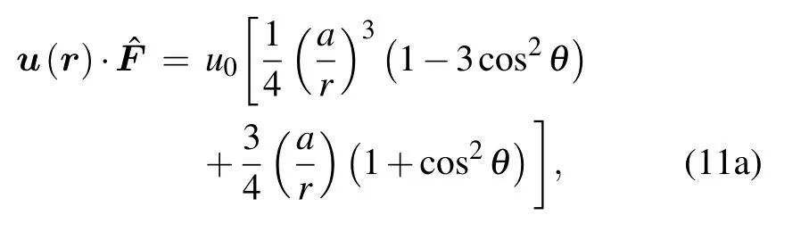
where u0denotes the particle velocity,r denotes the radial coordinate,and θ the polar angle defined relativeIn contrast, the Smoluchowski fluid velocity field for particle electrophoresis in the lab frame can be written as(see Section S2 in Supplementary material):

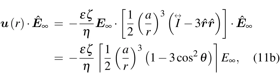
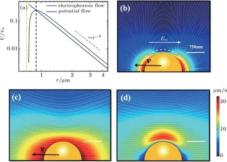
Fig. 3. Projected velocity and streamlines in the laboratory frame for same-sized particles under stationery condition (force balance with no acceleration). The white bars in the figures denote the length scale of 750 nm. (a)P2 projection of the electrophoretic velocity component along the electric field direction normalized by electrophoresis velocity v∞=μEE shows very good far-field 1/r3 behavior of the simulated velocity field,indicated by the red dashed line. Yellow dashed line shows the position of particle surface. Blue line shows the P2 projection of the Smoluchowski potential flow velocity field expressed by Eq.(11b). It is clear that the projected 1/r3 behavior stops at a small distance away from the solid surface.The peak position of the project result is delineated by the black dashed line,corresponding to the white dashed curve in panel(b). (b)Streamlines for the negatively charged PS sphere with a=0.75μm,(with λD=96.1 nm,κa=7.8,σ =7000 e/μm2)plotted in the lab frame. Here the colors indicate the magnitude of the velocity, the interface between the inner and outer flow fields (the reference surface) is denoted by white dashed curve. (c)Streamlines for a particle of the same radius as(a),acted on by a constant external body force to moves at same velocity asμEE∞. This represents the Stokes flow field in the lab frame. The contrast with the electrophoretic flow field shown in panel(b)is clear. (d)Streamline for the flow field obtained from a charged particle under the same electric field strength as in panel(b)but fixed by a reverse external(non-electrical)force acting on the particle. This flow field can also be obtained approximately by the superposition of the electrophoretic flow field in panel(b)and the Stokes flow field in panel(c)with a reversed velocity. It should be noted that the external(non-electrical)force required to immobilize the particle is not the same as the electrical force,thereby explaining the difference in the drag coefficients. The difference in the two forces accounts for the non-zero flow field close to the particle.

In Fig. 3(b) we show the full simulated electrophoretic flow field in the laboratory frame. It is noted that the streamlines of the electrophoretic flow pattern in Fig. 3(b) exhibits a belt of stationary vortices around the equatorial plane of the particle,with the electric field direction defining the north and south poles. The interface between the inner and outer flow fields is delineated here by the white dashed line. In contrast,in Fig.3(c)we show the Stokes flow field with the same-sized particle moving at the same velocity as in panel(b). There are no vortices in the flow field. The difference in the magnitude of the far field velocity is also apparent,as indicated by color,owing to the much slower 1/r velocity decay of the Stokes flow. Since the Reynolds number is negligibly small in electrophoretic flow,here the existence of vortices seen in Fig.3(b)is due to the large net charge and the associated strong local electric field in the Debye layer. It is known mathematically that the conditions for the existence of vortices are(i)the existence of a source term for vorticity (ω=?×v) as derived from the NS equation, and (ii) velocity reversal since the velocity on two sides of a vortex must be opposite. The latter condition is guaranteed in the laboratory frame of the electrophoretic flow close to the solid boundary and in the vicinity of the equatorial plane, because the electroosmotic flow induced by the net (positive) charge within the Debye layer is opposite to that of the solid particle.Hence both conditions are satisfied for the electrophoretic motion in the laboratory frame,but not in the co-moving frame due to the lack of velocity reversal. Hence vortices are not apparent for the electrophoretic motion in the co-moving frame. For the Stokes flow none of the two conditions is satisfied in the laboratory frame. Mathematical details for the non-inertial generation of vorticity,as in the present case,are shown in Section S6 in Supplementary material.

The physical manifestations of the inner flow field,as afforded by the full numerical solution of the relevant governing equations,represent a realization of the Smoluchowski picture in which the electroosmotic flow near the particle surface is the dominant mechanism of electrophoresis. In the original Smoluchowski solution(see Section S2 in Supplementary material)the inner flow field region was compressed to infinitesimal thickness for the sake of mathematical simplicity. Here we restore the inner flow field region with all its rich electrohydrodynamic flow behavior.

To further accentuate the difference between the electrophoretic and Stokes flows and their respective drag coefficients, in Fig. 3(d) we show the simulated flow field of a charged particle under the same applied electric field strength as in Fig.3(b)but fixed by an external non-electrical body force acting on the particle. This flow field can also be obtained approximately by the superposition of the electrophoretic flow field in Fig.3(b)and the Stokes flow field in Fig. 3(c) with a reversed velocity. The fact - that the flow field in panel 3(d) is not identically zero - emphasizes our point that the external non-electrical body force required to immobilize the particle is not the same as the electrical force.It also provides another, and perhaps more direct, explanation for why the drag coefficient in Eq.(1)is not the same as the electrophoretic drag coefficient. The difference between the Stokes versus the electrophoretic drag forces accounts for the non-zero flow field close to the particle in Fig.3(d), even though the net force is evaluated to be zero on the solid surface,as required by force balance on an immobile particle.

5. Closure between theory and experiment

5.1. Drag coefficient under differentκavalues

In Fig.4 we summarize the overall results of this work.In Fig.4(a)the ratio between the measured drag coefficients and the Stokes drag coefficient is plotted as open squares onto the solid simulation curves with different κa values, each evaluated on a surface at distance r outside the solid particle’s surface. The vertical dashed line indicates the inner/outer interface position,whose intersections with the different curves yield the drag coefficients at that interface. The measured results cluster around, and are close to, the values at the inner/outer interface. Their values are significantly smaller than the simulated values at the solid surface. The solid squares are calculated from the scaling argument［(4πa2)η/λD］/γS.[14,21]It is not surprising that these values at the solid surface are much larger than γS, since a/λDis in the range of 7-200 in our experimental measurements.

In Fig. 4(b) we plot the position of the inner/outer flow field interface,in terms of its dimensionless distance κΔ away from the particle surface, as a function of the salt concentration. Solid symbols indicate the inner/outer interface position as determined by the peak values in U/v∞as shown in Fig. 3(a). The open symbols represent the values of Δ determined by using measured drag coefficients as input to find the spherical surfaces on which the calculated drag forces exactly matches the measured values. Both the magnitudes and the trend of the empty symbols track the inner/outer interface position very well. Note that Δ is independent of surface charge density under a given particle radius.

The fact that the experimentally measured drag coefficient yields a surface position whose salt concentration dependence is identical to that of the inner/outer interface, ties the latter rather uniquely to its role as the reference surface for the electrophoretic drag and effective charge. Below we further reinforce this point by linking this inner/outer interface to the theoretical framework of O’Brien and White,[9]and Long et al.[21]

5.2. Dynamic simulation and comparison with measured data

To further substantiate the physical picture that the measured hydrodynamic drag coefficient should be evaluated by using the inner/outer interface (dashed white curve in Fig.3(b))as the reference(slip)surface/plane,we have carried out dynamic simulations by using the moving mesh approach.Details of the simulations are given in Section S6 in Supplementary material. In Fig.5 the open circles are the results of the dynamic simulation plotted as a function of time. The applied electric field is a step function with a very short rising time, shown in the inset. The dashed red curve is the fitting by using Eq.(12)below. In the absence of an optical trap,the dynamic equation of motion can be written as:

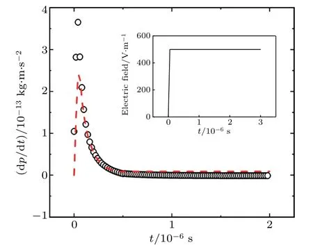
Fig.5. Momentum time derivative evaluated inside the inner flow field(including the solid particle) plotted as a function of time. Black circles are from dynamic simulation and red dashed curve is fitted from Eq.(12). Inset shows the corresponding electric field as a function of time.It shows a linear increase within 5×10-8 s to reach the saturation level.

For the left-hand side of Eq.(12),we sum up the momenta of the fluid and the solid at each finite element mesh within the inner/outer interface at each time step, and then evaluate its time derivative by using the data from successive time steps.The evaluation of the momenta is necessary since there are relative motions between the fluid and the solid. On the right hand side,the applied electric field is known,and for ˙x(t)we use the center of mass velocity of the evaluated unit. The two parameters γEand Qeffare then varied as the fitting parameters to best reproduce the simulation data. For a=0.75 μm and λD=96.1 nm, the best fit yields values of γE/γS=1.7 and |Qeff|=9.3×10-16C, they are in excellent agreement with the experimentally measured values of 1.69±0.27 and 9.1±1.4×10-16C, respectively. This indicates a consistent picture of drag coefficients evaluated from dynamic and static simulations,as well as consistency with the experimental measurements.

The fact that the inner flow field is carried along by the charged particle also means that the interface that separates the inner and outer flow fields represents a slip surface/plane.

5.3. Consistency between the framework of O’Brien and White, and Long et al., with the present theory and experimental results

We return to Eq. (1) and show that the inner flow field and its well-defined interface with the outer flow field constitute the missing piece in the theoretical framework of O’Brien and White,[22]and Long et al.,[21]that can tie together our theoretical predictions and the experimental results.

In a seminal paper, O’Brien and White simplified the governing equations for electrophoresis by assuming the coupled hydrodynamic and electric forces on a particle undergoing electrophoresis can be decoupled and solved separately.[22]The problem therefore becomes a superposition of two problems: the pure force problem (particle held fixed in a flow field with no applied field),and the pure electrophoresis problem (particle in an electric field in an electrolyte which is at rest at points far from the particle). Based on this analysis,Long et al.[21]showed that the velocity of the sphere is the sum of the two problems described above, based on global force balance:[14,21]

Here Felectricstands for the electric force, Fviscdenotes the viscous drag force, and Fextdenotes the non-electric external force. It should be reminded that v stands for the relative velocity between the particle and the far field fluid. Here equation(13a)is noted to be the same as Eq.(1).

Since we have demonstrated by using dynamic simulation that the inner flow field is carried along by the charged sphere, here we wish to use the inner/outer interface to evaluate all the relevant forces,so as to test Long et al.’s analysis while simultaneously also demonstrate the fact that γE/=γS.The latter can be seen from Eq. (13a) that, if Fext=0, then we must have v=μEE∞. When that happens, the force balance, equation (13b), becomes Feletric+Fvisc=0, i.e., a test of the electrophoretic drag also becomes possible since we can write Feletric=QeffE and Fvisc=γEv,both evaluated at the inner/outer interface.

All simulations were performed with surface charge density σ =-7×103e/μm2, particle radius a=0.75 μm, and ionic strength 0.01 mM(λD=100 nm).

To test Eqs. (13a) and (13b) at the interface that divides the inner and outer flow fields,Felectricin Eq.(13b)is the sum of electric forces inside the interface that divides the inner and outer flow fields. This force can be expressed as:

where ρ(r)=e[p(r)-n(r)]. On the other hand,Fviscstands for the drag force produced by the flow over the same inner/outer interface. It can be written as:

where σrrand σrθare the normal and tangential elements of the hydrodynamic stress tensor. From Eq. (13b), Fextis the negative of the sum of these two forces.

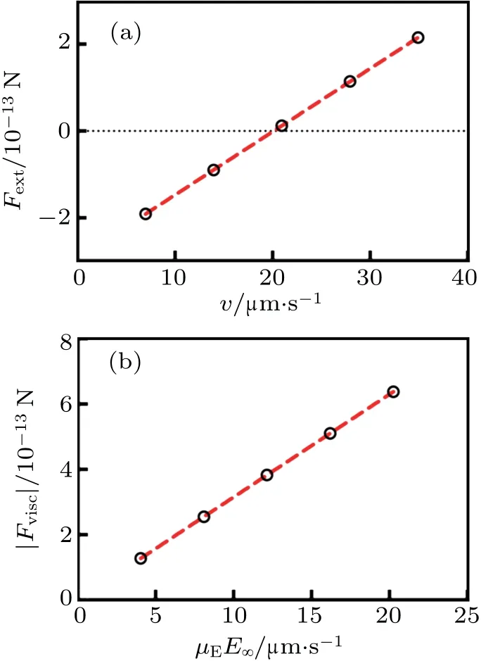
Fig.6. The difference between γS and γE,using Eq.(13). (a)External force Fext at interfacial region shows linear dependence with sphere velocity v. The open circles indicate five different values of v. The red dashed line denotes the best fitting with a slope 1.45×10-8 kg·s-1,which is very close to the Stokes drag coefficient 1.41×10-8 kg·s-1(=6πηa, 3% lower than the slope). The external force becomes zero when v is exactly at the electrophoretic velocity. The external electric field strength was maintained at E∞=500 V/m. (b)Viscous force Fvisc at interfacial region with sphere velocity v=μEE∞. The external electric field strength is varied from 100 V/m to 500 V/m in 100 V/m steps.The red dashed line indicates fitting with slope 2.9×10-8 kg·s-1(=2.1×6πηa). All simulations were performed with surface charge density σ =-7×103 e/μm2, radius a=0.75 μm, and ionic strength 0.01 mM(λD=100 nm).

By maintaining the solid particle stationary and varying the boundary value of the far field fluid velocity v,we evaluate the magnitude of Fextas a function of v,with the externally applied electric field maintained at E∞=500 V/m. We show in Fig.6(a)that the external force Fextdisplays a linear dependence on the relative velocity between the solid particle and the bulk fluid, with a slope given by 1.03γS. That is, equation(13a)is verified:

It should be noted that even though the net Fextis evaluated at r=a+Δ, the fact that the inner flow field is carried along by the solid particle implies the net force Fextto be the same as that evaluated at the center of mass of the particle,as well as at r=a.

In Fig.6(b), we focus on the case when Fext=0 so that Feletric=QeffE=Fvisc=γEv.By evaluating the viscous drag at the inner/outer interface and varying the external electric field strength from 100 V/m to 500 V/m in 100 V/m steps,we plot the resulting Fviscas a function of the electrophoretic velocity μEE∞. The slope gives a value that is 2.1 times the Stokes drag coefficient, which is somewhat higher than the experimentally measured value of γE/γS=1.7±0.3. However, both show unmistakable deviation from the Stokes drag coefficient. Therefore, we have explicitly used Long et al.’s analysis, based on the work of O’Brien and White, to show both the correctness of the equation Fext-γsΔv=0, as well as the necessary difference between the Stokes drag coefficient and the electrophoretic drag coefficient, both evaluated at the inner/outer interface.

6. Conclusions

We have measured electrophoresis drag coefficient γEby using an AC electric field to drive a charged particle in an optical trap. As far as we are aware, this is the first time such non-Stokes electrophoretic drag coefficients are determined experimentally. Our measurements were possible because our experimental arrangement permitted a time-varying electrophoretic motion of the charged particle with a speed directly proportional to that of the corresponding electric field strength.The non-electric, out-of-phase force from optical trap, fully counter-balanced by the out-of-phase electric force on the particle,does not play a role in hindering the electrophoretic motion. From both the experimental measurements and the direct numerical solutions, we show that the observed non-Stokes electrophoretic drag coefficient can be quantitatively described by the uniquely distinctive inner/outer interface as the reference plane for the evaluation of the hydrodynamic drag. The measured effective charge, Qeff, is consistent with the measured drag coefficient as required by force balance at the inner/outer interface flow fields which is at a distance a few λD’s away from the solid surface. The present experimental-theory study provides new,microscopic insights into the classic problem of electrophoresis. Such understanding can shed light on new applications of electrophoresis to investigate biological nanoparticles. More broadly, the experimental approach taken by this study and the microscopic view of an interface between the inner-outer flows might shed light to the outstanding problems of hydrodynamic forces and drags of other types of phoretic particles or swimming microorganisms.[41]

Acknowledgment

Ping Sheng wishes to acknowledge the funding support by Hong Kong RGC grants GRF16303415 and C6004-14G for this work.H.Daniel Ou-Yang wishes to acknowledge the support by US NSF grant 0923299 and the Emulsion Polymers Institute. Ping Sheng,Maijia Liao,and Shixin Xu wish to thank Chun Liu for advice regarding the necessary condition(s) for the appearance of hydrodynamic vortices. H.Daniel Ou-Yang and Ming-Tzo Wei would like to thank Kathryn Reddy,a former undergraduate student of Fordham University who participated in the initial experiments of this study during her REU at Lehigh. H.Daniel Ou-Yang would also like to thank Prof.Joel A.Cohen,Prof.Daan Frenkel,and Dr.Alois W¨urger for their critical comments and helpful suggestions.

Author contributions

Ping Sheng and H. Daniel Ou-Yang initiated and supervised the research. Maijia Liao and Ming-Tzo Wei carried out the experiments. Maijia Liao and Ping Sheng contributed to theory and simulations with help from Shixin Xu. Maijia Liao, H. Daniel Ou-Yang, and Ping Sheng analyzed the data with help from Ming-Tzo Wei. Maijia Liao,Ping Sheng,and H. Daniel Ou-Yang wrote the draft manuscript. All participated in revising the manuscript to its final form. Maijia Liao and Ming-Tzo Wei contributed equally to this work.