Multiple soliton solutionsforthe(3+1)conformable space–time fractional modi fi edKorteweg–de-Vriesequations

R.I. Nuruddeen

Department of Mathematics, Federal University Dutse, Dutse, Jigawa State, Nigeria

1.Introduction

Nonlinear partial differential equations are known for their vital roles in many science and engineering application problems such as in the hydrodynamics, fl uid mechanics, plasma physics and nonlinear dispersive wave among others. These dispersive waves emanate from the problems of shallow water waves. However, a very good example of the nonlinear partial differential equation describing shallow water waves is the Korteweg–de-Vries equation (KdV) [1] given by

The KdV equation also plays role in modeling blood pressure pulses and internal gravity waves in oceans among others. Thus, investigating such exact traveling wave solutions attached to this problem is paramount since they help in understanding the physics behind. In addition, as higher dimensional models turn to be more realistic; several modi fi cations to Eq. (1) have been proposed in literature among which the (3+1)-dimensional modi fi ed KdV equation given in Eq.(2) by Hereman [2,3] and the recent (3+1)-dimensional modi fi ed KdV equations given in Eqs. (3) and (4) by Wazwaz[4] that read

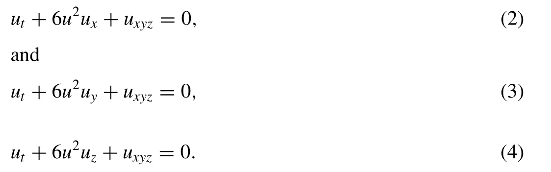
These equations play important role in three-dimensional nonlinear dispersion problems. However, this paper aims to study this modi fi ed KdV equations given in Eqs. (2) –(4) with the introduction of the fractional order derivative in both the space and time variables using the new conformable fractional derivative [5] . Also, it would be good to note that several analytical methods have been used in this regard in treating such problems, read [6–35] .

The de fi nition of the conformable fractional derivative[5] read; letu: [0,∞)→ R,theα′s order conformable derivative ofuis de fi ned by

The paper is organized as follows: Section 2 devoted to properties of the conformable fractional derivative and method. Section 3 tackles the main problems. In Section 4 ,we give the graphical representations and discussion and Section 5 is for conclusion.

2.The properties of the conformable fractional derivative and methodology of solution

Some properties of the conformable fractional derivative are given using the following de fi nition:

De fi nition:Letα∈ (0, 1] and supposeu(t) andv(t) areα-differentiable att＞0. Then

(a)c)=ctc-α,for allc∈ R.

(b)(a)= 0,afor all constant functionu(t)=a.

(c)(au(t))=for allaconstant.

(d)(au(t)+bv(t))=+for alla,b∈R.

(g) If in addition tou(t) is differentiable, then

Now, considering the following conformable fractional differential equation, we present the method:

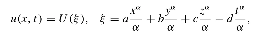
By the wave transformation, we set

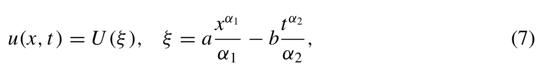
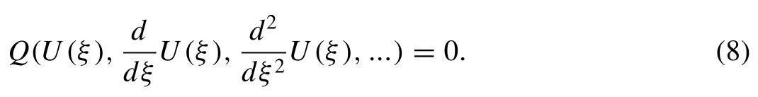
whereα1,α2are fractional orders,aandbare nonzero constants. Substitution of transformation (7) into Eq. (6) , we get a reduced ordinary differential equation of the polynomial form

Then, we assume the solution of the fi nite series of the form given by:

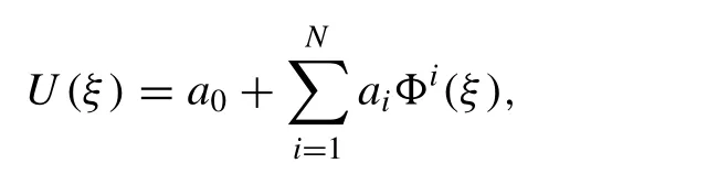
where,a0,a1,a2, ...,aNare constants.Nis positive integer determined by homogeneous balancing method andΦ(ξ) is purposely chosen in this work to be sech(ξ) andcosech(ξ)in the case of hyperbolic function solutions while sec(ξ)and cosec(ξ) in the case of periodic functions solutions, respectively.

3.Application

In this section, we present some hyperbolic and periodic solutions for the (3+1)-dimensional conformable space–time fractional modi fi ed Korteweg–de-Vries (mKdV) equations.

3.1. The fi rst conformable space–time fractional mKdV equation

We consider the fi rst (3+1)-dimensional conformable space–time fractional mKdV equation given by

Applying the wave transformation,

we get

On integrating Eq. (10) once with zero constant of integration assumption, we get

Also, by homogeneous balancing method we determineN= 1 from Eq. (11) .

3.1.1.Hyperbolicsolutions

To determine the hyperbolic solutions for the fi rst (3+1)-dimensional conformable space–time fractional mKdV equation given in Eq. (9) , we seek solutions of the form

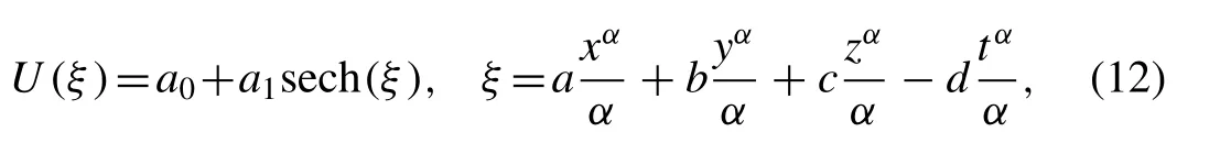
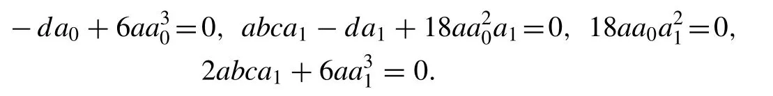
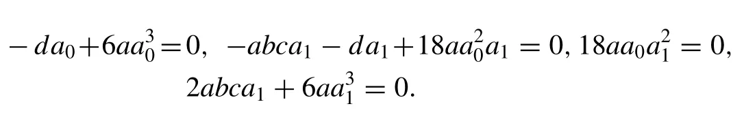
where,a0,a1,a,b,canddare constants to be determined.Substituting Eq. (12) into Eq. (11) , equating the coef fi cients of sechj(ξ),j= 0,1,2,3 to zero we get the algebraic equations with the help of Mathematica software as follows:

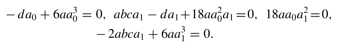
Solving the above algebraic equations yields:

= 0,d=abc,which produce the solutions:

(see Fig. 1 (a) and (b)).

For more hyperbolic solutions, we again seek a solution of the form

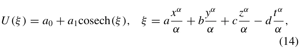
Substituting Eq. (14) into Eq. (11) , equating the coef fi cients of cosechj(ξ),j= 0,1,2,3 to zero we get the algebraic equations with the help of Mathematica software as follows:

Solving the above algebraic equations yields:

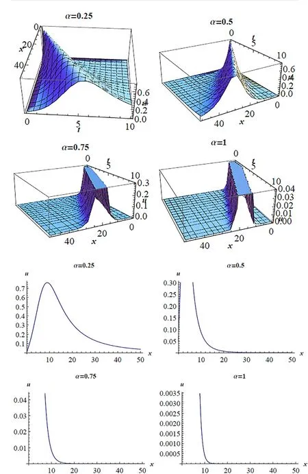
Fig. 1. (a) 3D pro fi les for Eq. (13) on subsituting the values of the parameters a = 0.5 7, b = = -2 , z = 3, t = 10;α= 0. 57, 0. 9. (b) 2D pro fi les for Eq. (13) on subsituting the values of the parameters a = 1, b == 1 , y = 0, z = 0, t = 1 at various α′s .

ad=abc,which produce the solutions:

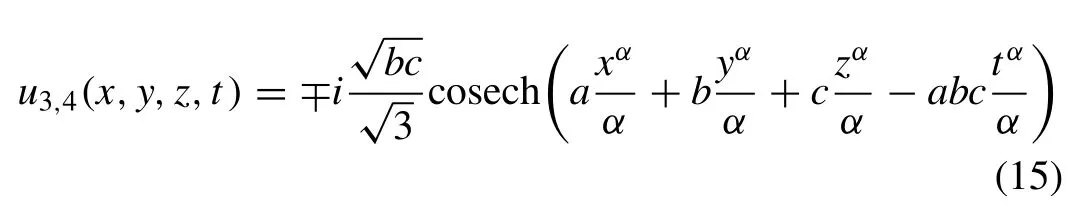
(see Fig. 2 (a) and (b)).

3.1.2.Periodicsolutions

To determine periodic the solutions for the fi rst (3+1) dimensional conformable space–time fractional mKdV equation given in Eq. (9) , we seek solution of the form

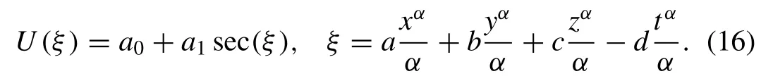
Substituting Eq. (16) into Eq. (11) , equating the coef fi cients of secj(ξ),j= 0,1,2,3 to zero we get the algebraic equations with the help of Mathematica software as follows:

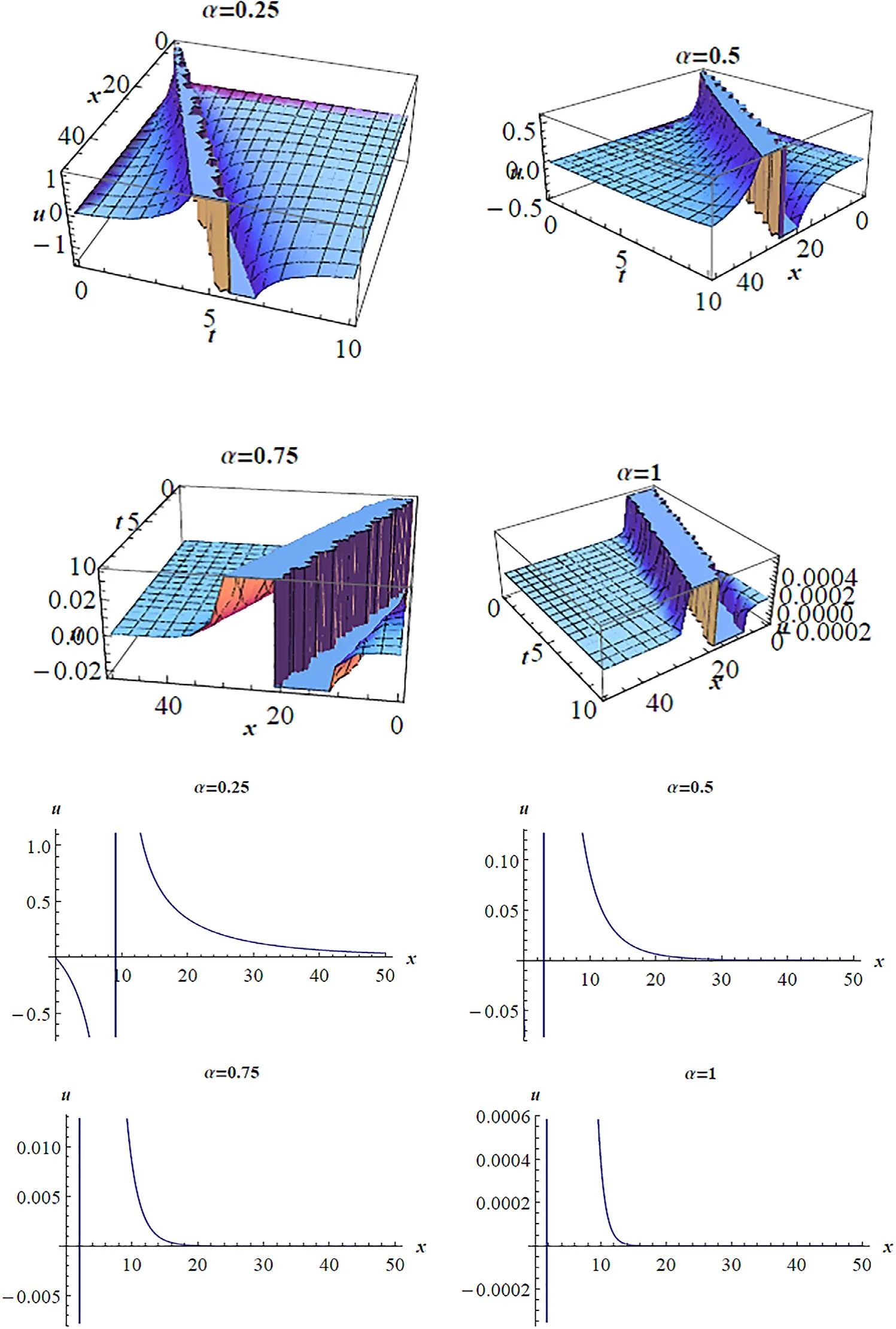
Fig. 2. (a) 3D pro fi les for Eq. (15) on subsituting the values of the parameters a = 1, b = c = 1 , y = 0, z = 0 at various α′ s. (b) 2D pro fi les for Eq.(15) on subsituting the values of the parameters a = 1, b == 1, y = 0, z = 0, t = 1 at various α′s.

And solving the algebraic equations yields:

ad= -abc, which produce the solutions:

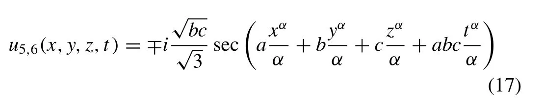
(see Fig. 3 (a) and (b)).

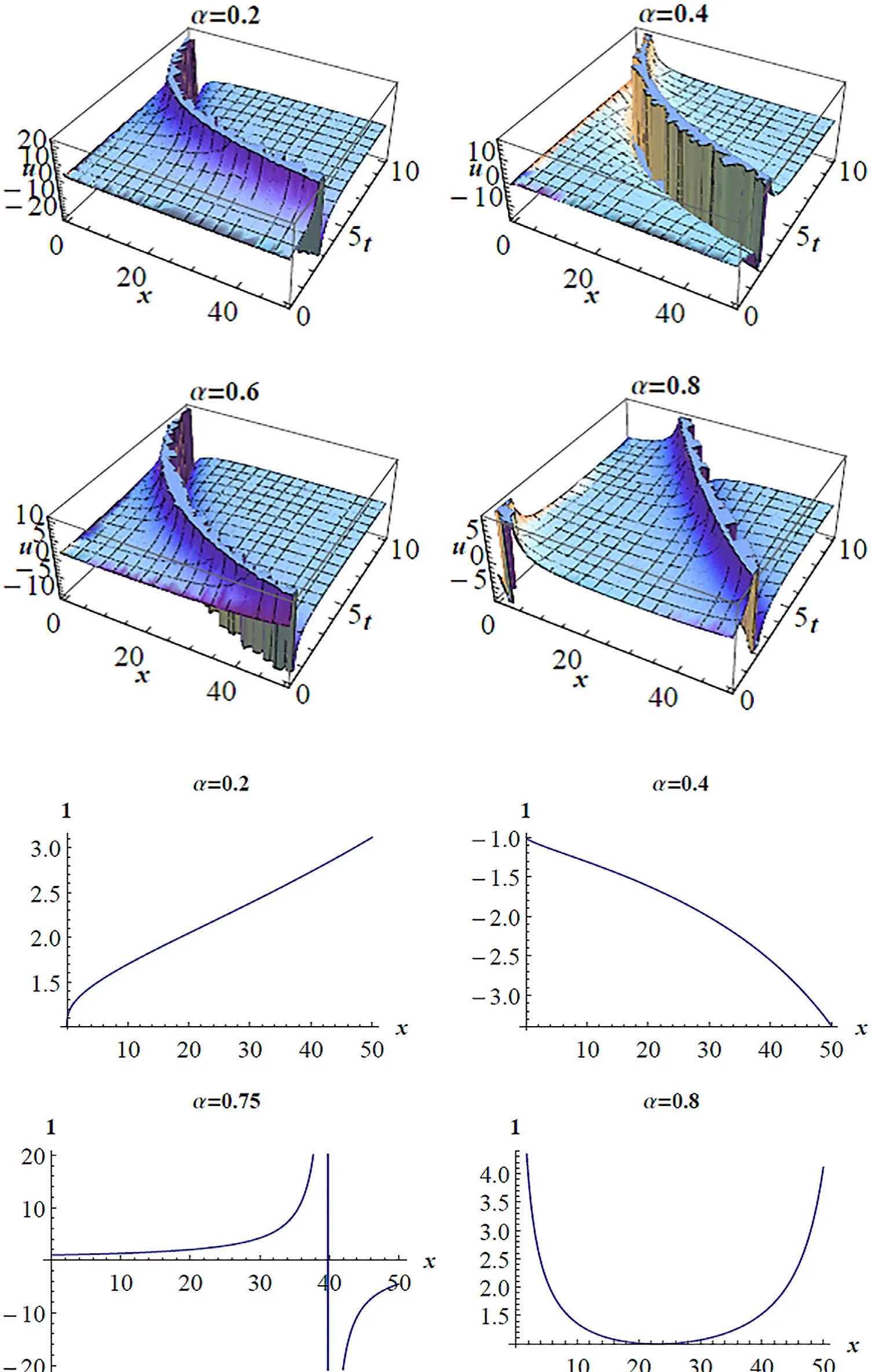
Fig. 3. (a) 3D pro fi les for Eq. (17) on subsituting the values of the parameters a = 0. 1 , b = 2, c = 1 . 5 , y = 1 , z = 1 at various α′ s . (b) 2D pro fi les for Eq.(17) on subsituting the values of the parameters a = 0. 1 , b = 2, c = 1 . 5 , y = 1 , z = 1 , t = 1 at various α′ s .

In the same way, we seek again a periodic solution of the form

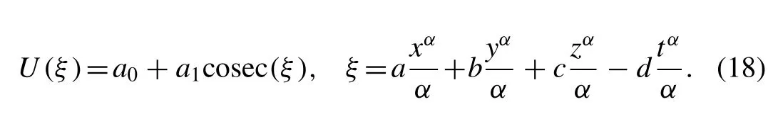
Substituting Eq. (18) into Eq. (11) , equating the coef fi cients of cosecj(ξ),j= 0,1,2,3 to zero we get the algebraic equations with the help of Mathematica software as follows:

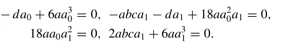
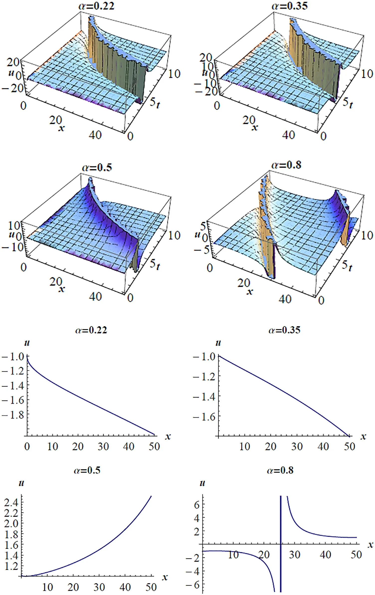
Fig. 4. (a) 3D pro fi les for Eq. (19) on subsituting the values of the parameters a = 0. 1 , b = 2, c = 1 . 5 , y = 1 , z = 1 at various α′ s . (b) 2D pro fi les for Eq.(19) on subsituting the values of the parameters a = 0. 1 , b = 2, c = 1 . 5 , y = 1 , z = 1 , t = 1 at various α′ s .

And on solving the above system we get:

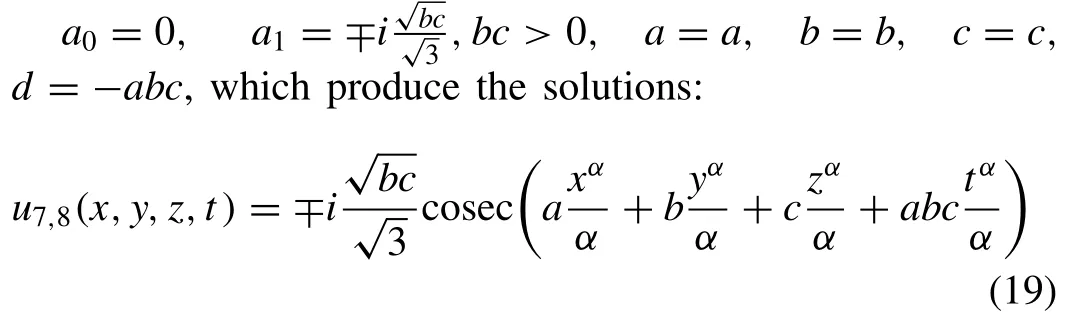
(see Fig. 4 (a) and (b)).

3.2. The second conformable space–time fractional mKdV equation

We consider the second (3+1)-dimensional conformable space–time fractional mKdV equation given by

Proceeding as before gives the following set of solutions.

3.2.1.Hyperbolicsolutions

3.2.2.Periodicsolutions

3.3. The third conformable space–time fractional mKdV equation

We consider the third (3+1)-dimensional conformable space–time fractional mKdV equation given by

Proceeding as before gives the following set of solutions.

3.3.1.Hyperbolicsolutions

and

3.3.2.Periodicsolutions

4.Graphical representation and discussion

In this section, we give the 3-dimensional representations(3D) and the 2-dimensional representations (2D) of the fi rst(3+1)-dimensional conformable space–time fractional mKdV equation in Figs. 1–4 ((a) and (b)). Different soliton solutions are plotted ranging from soliton solutions shapes, singular soliton solutions and periodic type wave solutions at different values ofαas stated in each fi gure. In addition, similar graphical representations can be plotted for the remaining second and third (3+1)-dimensional conformable space–time fractional mKdV equations, respectively.

5.Conclusion

In conclusion, the old and the newly introduced (3+1)-dimensional modi fi ed Korteweg–de-Vries equations (mKdV)by [4] are analyzed in the present coupled with the introduction of the conformable fractional derivative orders in both the space and time variables. A variety of soliton solutions ranging from hyperbolic to periodic function solutions are constructed for the equations under consideration. Also,the present solutions serve as new solutions to the modi fi ed Korteweg–de-Vries equation (mKdV) considered in Wazwaz[4] atα= 1 . Finally, the Mathematica software is utilized throughout for the solution and graphical representations.

[1] R. Hirota , J. Satsuma , Phys. Lett. A 85 (1981) 407–408 .

[2] W. Hereman , Exact solutions of nonlinear partial differential equations the tanh/sech method, Wolfram Research Academic Intern Program Inc.,Champaign. Illinois, 2000, pp. 1–14 .

[3] W. Hereman , Shallow water waves and solitary waves, encyclopedia of complexity and systems science, Springer Verlag, Heibelberg, Germany,2009, pp. 8112–8125 .

[4] A.M. Wazwaz , DE GRUYTER. Open Eng. 7 (2017) 169–174 .

[5] R. Khalil , et al. , J. Comput. Appl. Math. 264 (2014) 65–701 .

[6] N. Kudryashov , Commun. Nonlinear Sci. Numer. Simul. 17 (11) (2012)2248–2253 .

[7] K.R. Raslan , K.A. Khalid , M.A. Shallal , Chaos Solitons Fract. 103(2017a) 404–409 .

[8] K.R. Raslan , S.E. Talaat , K.A. Khalid , Eur. Phys. J. Plus 132 (319)(2017b) .

[9] K.R. Raslan , S.E. Talaat , K.A. Khalid , Commun. Theor. Phys. 68 (1)(2017c) 49–56 .

[10] K. Hosseini , A. Bekir , R. Ansari , Opt. Quantum Electron. 49 (131)(2017) .

[11] R.I. Nuruddeen , A.M. Nass , Stochastic Modell. Appl. 21 (1) (2017)23–30 .

[12] A.E. Bekir , O.A. Guner , Int. J. Nonlinear Sci. Numer. Simul. 15 (2014)463–470 .

[13] M. Matinfar , M. Eslami , M. Kordy , Pramana J. Phys. 85 (2015)583–592 .

[14] H.C. Yaslan , Int. J. Light Electron Opt. 140 (2017) 123–126 .

[15] E. Fan , Phys. Lett. A 277 (2000) 212–218 .

[16] Z. Fu , et al. , Phys. Lett. A 290 (2001) 72–76 .

[17] S.M.R. Islam , K. Khan , K.M.A. Woadud , Waves Random Complex Media (2017) 1–10 .

[18] A. Biswas , et al. , Indian J. Phys. 87 (2) (2013) 169–175 .

[19] R.I. Nuruddeen , Sohag J. Math. 4 (2) (2017) 1–5 .

[20] Z. Yan , H.Q. Zhang , Phys. Lett. A 285 (2001) 355–362 .

[21] A.R. Seadawy , D. Lu , M.M.A. Khater , J. Ocean Eng. Sci. 2 (2017)137–142 .

[22] M. Saad , et al. , Int. J. Basic Appl. Sci. 13 (1) (2013) 23–25 .

[23] T. Elghareb , et al. , Int. J. Basic Appl. Sci. 13 (1) (2013) 19–22 .

[24] J. Mana fi an , M. Lakestani , Optik 127 (2016) 2040–2054 .

[25] M.M. Hassan , et al. , Rep. Math. Phys. 74 (2014) 347–358 .

[26] H. Bulut , et al. , Eur. Phys. J. Plus 132 (350) (2017) 1–12 .

[27] H. Bulut , et al. , Opt. Quantum Electron. 48 (1) (2016) .

[28] H.M. Baskonus , T.A. Sulaiman , H. Bulut , Indian J. Phys. 132 (2017)482 .

[29] R.I. Nuruddeen , L. Muhammad , A.M. Nass , T.A. Sulaiman , Palestine J.Math. 7 (1) (2017) 262–280 .

[30] S.M.R. Islam , K. Khan , M.A. Ali , Exact solutions of unsteady Korteweg-de Vries and time regularized long wave equations, Springer Plus, 2015 .

[31] K. Khan, M.A. Ali, S.M.R. Islam, 2014, 3(724), Springer Plus.

[32] S.M.R. Islam , K. Khan , M.A. Ali , Brit. J. Math. Comput. Sci. 5 (3)(2014) 397–407 .

[33] D. Baleanu , M. Inc , A.I. Aliyu , A. Yusuf , Int. J. Light Electron Opt.147 (2017) .

[34] M. Inc , A. Yusuf , A.I. Aliyu , Opt. Quantum Electon. 49 (11) (2017) .

[35] M.I. Syam , H.M. Jaradat , M. Alquran , Nonlinear Dyn. 89 (2) (2017) .