Assessment of ship manoeuvrability by using a coupling between a nonlinear transient manoeuvring model and mathematical programming techniques*

TRAN KHANH Toan, OUAHSINE Abdellatif

Laboratoire Roberval, Université de Technologie de Compiègne, UTC-CNRS 7337, CS 60319, 60206 Compiègne cedex, France, E-mail: toantk.ctt@vimaru.edu.vn

NACEUR Hakim

Laboratoire Roberval, Université de Technologie de Compiègne, UTC-CNRS 7337, CS 60319, 60206 Compiègne cedex, France

Laboratoire LAMIH, Université de Valenciennes, UMR 8201 CNRS, 59313 Valenciennes, France

EL WASSIFI Karima

Université Cadi Ayyad, Faculté des Sciences et Techniques, BP 549, Marrakech, Morocco

(Received June 17, 2013, Revised August 15, 2013)

Assessment of ship manoeuvrability by using a coupling between a nonlinear transient manoeuvring model and mathematical programming techniques*

TRAN KHANH Toan, OUAHSINE Abdellatif

Laboratoire Roberval, Université de Technologie de Compiègne, UTC-CNRS 7337, CS 60319, 60206 Compiègne cedex, France, E-mail: toantk.ctt@vimaru.edu.vn

NACEUR Hakim

Laboratoire Roberval, Université de Technologie de Compiègne, UTC-CNRS 7337, CS 60319, 60206 Compiègne cedex, France

Laboratoire LAMIH, Université de Valenciennes, UMR 8201 CNRS, 59313 Valenciennes, France

EL WASSIFI Karima

Université Cadi Ayyad, Faculté des Sciences et Techniques, BP 549, Marrakech, Morocco

(Received June 17, 2013, Revised August 15, 2013)

In this paper, a numerical method based on a coupling between a mathematical model of nonlinear transient ship manoeuvring motion in the horizontal plane and Mathematical Programming (MP) techniques is proposed. The aim of the proposed procedure is an efficient estimation of optimal ship hydrodynamic parameters in a dynamic model at the early design stage. The proposed procedure has been validated through turning circle and zigzag manoeuvres based on experimental data of sea trials of the 190 000-dwt oil tanker. Comparisons between experimental and computed data show a good agreement of overall tendency in manoeuvring trajectories.

ship manoeuvrability, hydrodynamics coefficients, nonlinear transient dynamics, sensitivity analysis, mathematical programming

Introduction

Controlling ship manoeuvrability, especially when approaching ports in foggy weather or by night time, is a vital concern. Nowadays, it is still tedious to perform real ship manoeuvres in an open sea or to carry out fine simulations using complex 3-D CFD calculations. In spite of their fast calculations, systembased simulations need numerous tests to adjust the manoeuvring hydrodynamic coefficients (hull, rudder, propeller,...) in order to achieve quantitative agreement with the experimental measurements. In this context, manoeuvrability turns out to be an essential ability to perform a safe navigation of any ship against the danger of collisions and stranding.

Thus, enhancement of ship manoeuvrability in different approaches is introduced more and more in the early design stage of ships and vessels. It is important to understand the ship manoeuvrability in the early design stage. In order to force the vessel motion to follow a prescribed trajectory, accurate prediction of hydrodynamic forces acting on a ship hull and interaction among them, propeller and rudder is essential. A literature survey[1-3]showed that there exist three methods for ship manoeuvrability prediction: the experiment-based method, the system-based method and the CFD-based method. A general overview of methods for ship trajectory prediction is given in Fig.1.

Manoeuvring experiments can be accomplished in two different ways, depending on the testing purpose, facilities and equipment, as free sailing or captive model tests. Objectives of manoeuvrability test are: the verification of manoeuvrability to fulfill theInternational Maritime Organization (IMO) criteria, and the determination of hydrodynamic manoeuvring coefficients. Although this method is effective, unfortunately, experimental determination of the hydrodynamic coefficients might be tedious and expensive.

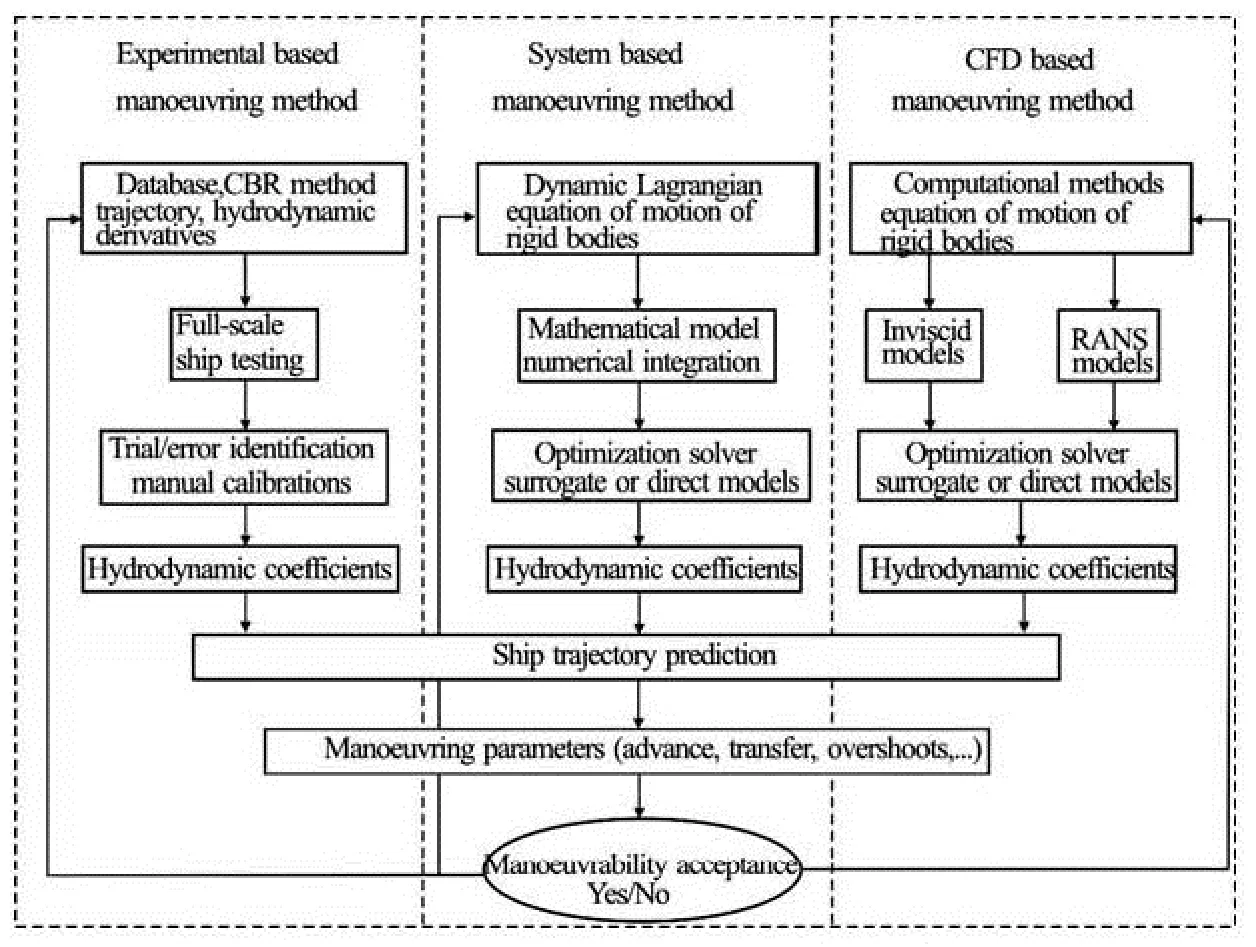
Fig.1 Overview of methods for ship trajectory prediction

The CFD–based method allows determining not only the motion of the ships but also the flow field around ships by solving a set of Reynolds-Averaged Navier-Stokes (RANS) equations[3,4]. Lately, the CFD–based method has been extended for free-running simulations, including measurable data from experimental fluid dynamics for ship manoeuvres in calm sea and in the presence of waves. In their numerical investigations, Fonfach et al.[5]used CFD with both free surface model and rigid wall free surface assumption to study the interaction between a smaller tug and a larger tanker moving in parallel and close to each other at low speed in shallow water. For surge force, sway force and yaw moment in different water depths andFr, they showed that CFD results give better agreement with experimental fluid dynamics than available Potential Flow (PF) results.

The system–based method is a major simulation task to predict ship manoeuvrability[2]. Computation time is much shorter than that of CFD–based method since such method needs only solve the equations of motion using a prescribed mathematical model and manoeuvring coefficients. System–based method requires approximately a few minutes of computation on a personal computer for one free-running trial while CFD method needs a few hours or even days depending on the turbulence and propulsion modeling and the mesh size.

System–based methods have been extensively investigated by researchers[6-8]. A simplified mathematical formulation can be obtained by using Taylor’s series expansion method. The course keeping stability of the ship can be investigated on the basis of the stability of the solutions of the linear equations of motion, if only first-order terms of this expansion are considered. However, the manoeuvres at high rudder deflection angles require the consideration of nonlinear hydrodynamic and inertial components. This leads to the utilization of nonlinear hydrodynamic models, which include higher-order terms of Taylor’s series expansion of the hydrodynamic external forces and moments[6].

Generally the manoeuvring coefficients are supposed to be constant. Nonetheless, recently Araki et al.[3]showed a great disparity of manoeuvring coefficients when including waves in which the encounter frequency is low. The complexity of the hydrodynamic processes caused by the wide variety of ship shapes, sizes and motions leads to a multitude of mathematical models. Thus, to obtain an optimized trajectory and also a better understanding of ship manoeuvring it is necessary to improve the understanding of the hydrodynamic forces acting on the hull, the rudder and the propeller. Several mathematical models of dynamic ship motion have been proposed in the literature to identify the hydrodynamic parameters[9,10]. Yoon and Rhee[11]investigated a mathematical model based on the Estimation-Before-Modeling (EBM) technique, which is an identification method that estimates parameters in a dynamic model. The algorithm was validated using real sea trial data of a 113 K tanker. Viviani et al.[12]carried out a numerical study based on optimization techniques that used a Multi-Objective Genetic Algorithm (MOGA). They identified five most sensitive hydrodynamic coefficients from standard manoeuvres (specified by the IMO) for a series of twin-screw ships. Rajesh and Bhattacharyya[13]conducted a numerical study based on system identification for a nonlinear manoeuvring model dedicated for large tankers by using the artificial neural network method. In this model, all nonlinear terms are set together to form one unknown time function per equations which are sought to be represented by the neural network coefficients. Seo and Kim[14], performed a numerical analysis of ship manoeuvring performance in the presence of incident waves and resultant ship motion responses. To this end, a time domain ship motion program was developed to solve the wave body interaction with the ship slip speed and rotation, and coupled to a modular type 4DOF manoeuvring model. Zhang and Zou[15]analyzed the data of longitudinal and transverse velocity, rudder angle, etc. in the simulated zigzag test. This paper presents an efficient procedure to determine optimal hydrodynamic coefficients by using a mono-objective optimization based on a Mathematical Programming (MP) technique suitable for highly nonlinear problems such us ship manoeuvring simulation from sea trials. Accurate modeling of a ship trajectory is achieved effectively using the following three steps. The first step deals with the modeling of the nonlinear dynamic ship motion, to this end a 3DOF mathematical model based on the Lagrangian dynamic motion of a 3-D rigid body has been developed taking into account the nonlinear hydrodynamic forces acting on the ship hull, propeller and rudder. Then a sensitivity analysis is carried out to identify the most significant hydrodynamic coefficients affecting the ship trajectory. The interest of applying sensitivity analysis is to reduce the number of coefficients to be optimized. Therefore the hydrodynamic model can be easily treated using a constrained mono-objective minimization procedure. In the present investigation, it is found that only 14 coefficients are sensitive for the prediction of the trajectory of the ESSO 199 000-dwt oil tanker benchmark[7]. The obtained results have been validated through turning circle and zigzag manoeuvres based on experimental data of sea trials of the above-cited benchmark. The last step of the proposed procedure concerns the determination of optimal hydrodynamic parameters using MP techniques[16,17]. To date, based on our knowledge, the MP techniques based identification has not been studied in the context of the manoeuvring of large tankers. The present paper makes an attempt to do so for the first time. A summary of the MP based system identification for the identification of optimal hydrodynamic coefficient is given in Table 1.

The structure of the paper is as follows. First, the dynamics of ship motion and hydrodynamic forces in coupled equations (the so-called hydrodynamic model), are explained in Section 1. Section 2 presents the mathematical programming based system identification for manoeuvring of large tankers. In Section 3 numerical applications are exposed and the obtained results are analyzed and compared to the experimental measurements. Finally, conclusions are drawn in Section 4 to summarize the present investigation.

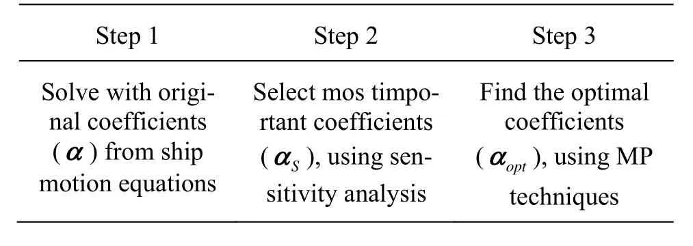
Table 1 Summary of MP based system identification

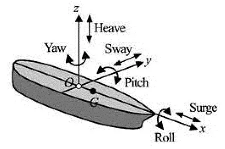
Fig.2 Ship motion in 6 DOF

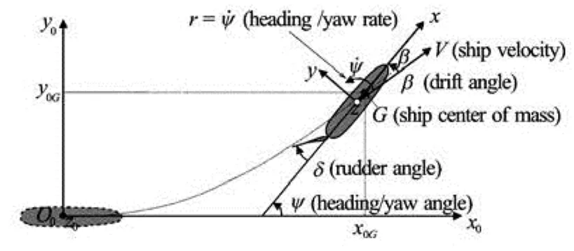
Fig.3 Definition of the coordinate system, speed and direction

1. Formulation of the nonlinear transient hydrodynamic model

1.1Lagrangian based dynamic equation of 2-D ship manoeuvring motin in the horizontal plane

In the manoeuvring theory, we use the coordinate systemOxyz(see Fig.2), fixed to the rigid body of the ship.Gis the center of mass andOxzis a plane of symmetry. The space fixed system isO0x0y0z0as shown in Fig.3. The ship motion has six degrees of freedom (6 DOF). The Euler angles describing the position of the ship axes are the heading or yawψand the rollφ. The angle between the directions ofx0axis andxaxis is defined as the heading angleψ. During manoeuvring, the position of the ship can be obtained by the coordinates (x0G,y0G) of the ship center of mass in the global coordinate systemO0x0y0z0, and the orientation of the ship is obtained by the heading angleψ(see Fig.3).

The transient ship manoeuvring motion in the horizontal plane can be described by the translational velocityVand the yaw rater=ψ˙ of the rotational motion around theOzaxis (see Fig.3). The instantaneous cartesian components of the velocityVin the mobile coordinate systemOxyzareuin thex-axis direction andvin they-axis direction, respectively. The angle between the direction of velocityVand the ship axisOxaxis is defined as the drift angleβ.

According to the Newton second law, the nonlinear transient equations of motion in the ship moving coordinate systemOxyzcan be written in the form[18]

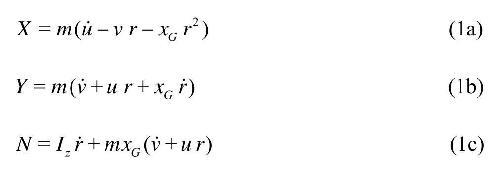
wheremis the mass of the ship,XandYthe external forces,Nthe external moment,Izthe moment of inertia about thezaxis,rthe heading/yaw, (xG, 0,zG) are the coordinates of the center of massG.

Generally it is more suitable to use the non-dimensional form of the dynamic equations of motion. Dividing the first two equations of (1) bymgand the last equation bymgL, wheregis the gravity acceleration andLis the ship length, we obtain the linear equations of ship manoeuvring motion

where=L-1(/m)1/2is the non-dimensional radius of gyration andx=X/mg,y=Y/mg,N=N/mgLare the non-dimensional forces and moment respectively.

1.2Formulation of the hydrodynamic forces

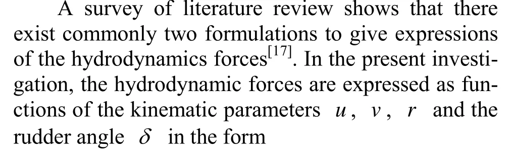
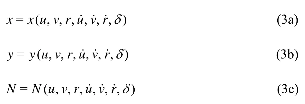
By using an expanded Taylor series to the second order, about the steady state of forward motion, and by maintaining only most influencing physical terms, one can obtain the following expressions of the nonlinear hydrodynamic forces and moment[19]:

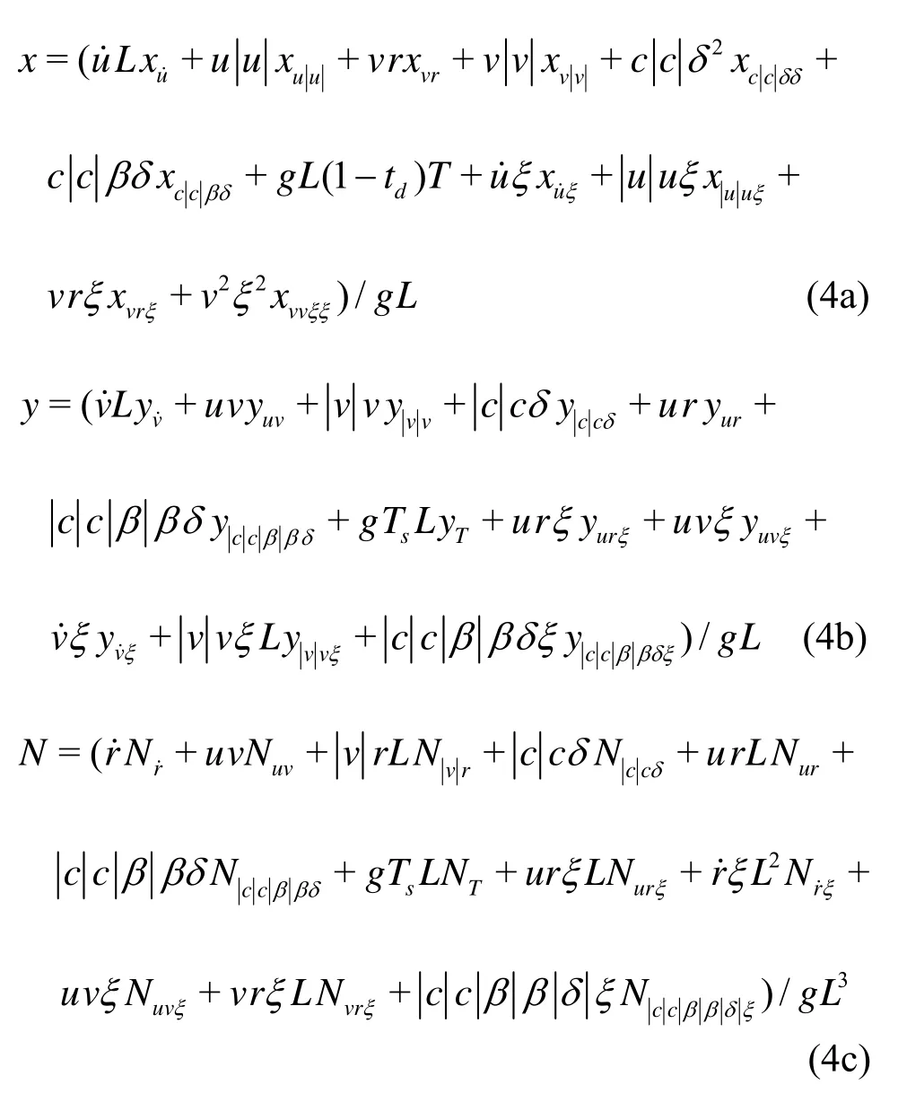
whereβis the ship drift angle,xu˙,xuu,…,yu˙,yuv,…,Nr˙,Nuv,…,Nccββδξare the non-dimensional derivatives of ship hydrodynamic coefficients, which have to be identified,tdis the thrust deduction coefficient,β=-v/u,ξ=Ts/(h-Ts) whereTsis the ship draft,his the water depth. The non-dimensional propeller thrustTis given by

whereTuu,TunandTnnare the hydrodynamic coefficients andnis the shaft velocity.

The flow velocitycat the rudder is estimated by

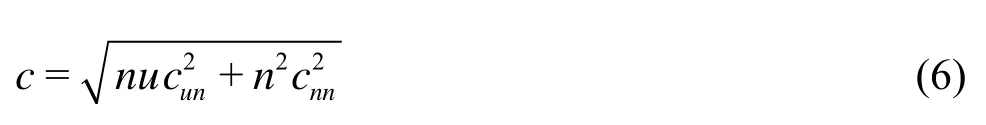
wherecunandcnnare the hydrodynamic coefficients.

1.3Numerical integration of the nonlinear transient equations

In order to solve the manoeuvring problem, the nonlinear Ordinary Differential Equations (ODE) given in Eq.(2) have to be solved using appropriate numerical integration schemes. A stable and accurate integration of nonlinear ODE is of great importance for the solution of the transient equations of motion.

For this purpose, we first define a set of primary variablesxdescribing entirely the manoeuvrability, which can be composed of: the ship velocity componentsu,v,r, the ship position componentsx0,y0,ψin the global cartesian coordinate systemO0x0y0z0, the actual rudder angleδand the shaft instantaneous velocityn. This may be written as

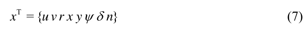
The complete manoeuvrability of ship is carried out by assemblying and solving the set of ODE given by Eq.(2), the yaw rateψ?=rand the rates ?δ, ?nof rudder angle and the shaft velocity, respectively.

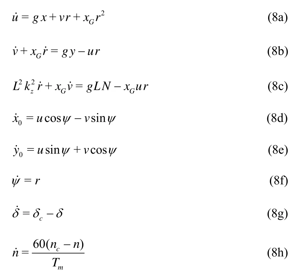
whereTmis the coefficient of propeller,cδthe commanded rudder angle, andncis the commanded shaft velocity. Equation (8) can be rewritten in a more simple form, function of the state variables of ship motion, leading to a nonlinear time-varying system.

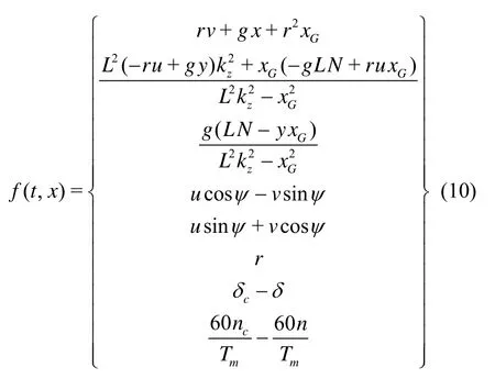
withtdenoting the time.

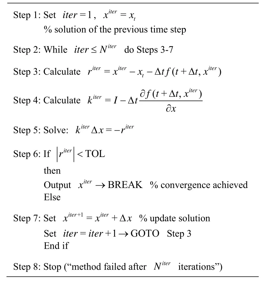
Table 2 Procedure used in the implicit Euler integration scheme

1.3.1 Implicit Euler scheme

A first approach to the discrete approximate solution of Eq.(9), assuming thatfis sufficiently differentiable with respect totandx, is to express Eq.(9) at timet+Δtby

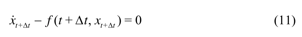
Then the time derivative ofxat timet+Δtis approximated using the Euler backward finite difference formula

It is noted that other more sophisticated numerical schemes may be used[18].

By substituting formula (12) into formula (11), we obtain the final implicit Euler prediction/correction procedure.

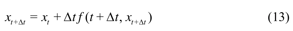
Equation (13) represents a system of nonlinear equations inxt+Δt, and a Newton-Raphson (NR) procedure should[20]be used at every time step to findxt+Δt. By denotingr=xt+Δt-xt-Δtf(t+Δt,xt+Δt) the residual vector from Eq.(13), the general NR iterative procedure is shown in Table 2.

It is worth noting that the proposed NR iterative procedure given in Table 2 converges in 3 to 4 iterations, which is no time consuming, and that the Euler implicit scheme is unconditionally stable.

1.3.2 Runge-Kutta scheme

The Euler scheme is not so useful because of its low accuracy. It is possible to use one step methods that match the accuracy of the higher-order Taylor series expansions by sequentially computing the functionf(t,x) at several points within the time interval. One of the most widely used Runge-Kutta (RK) methods is the fourth order method which requires four function evaluations per time step.

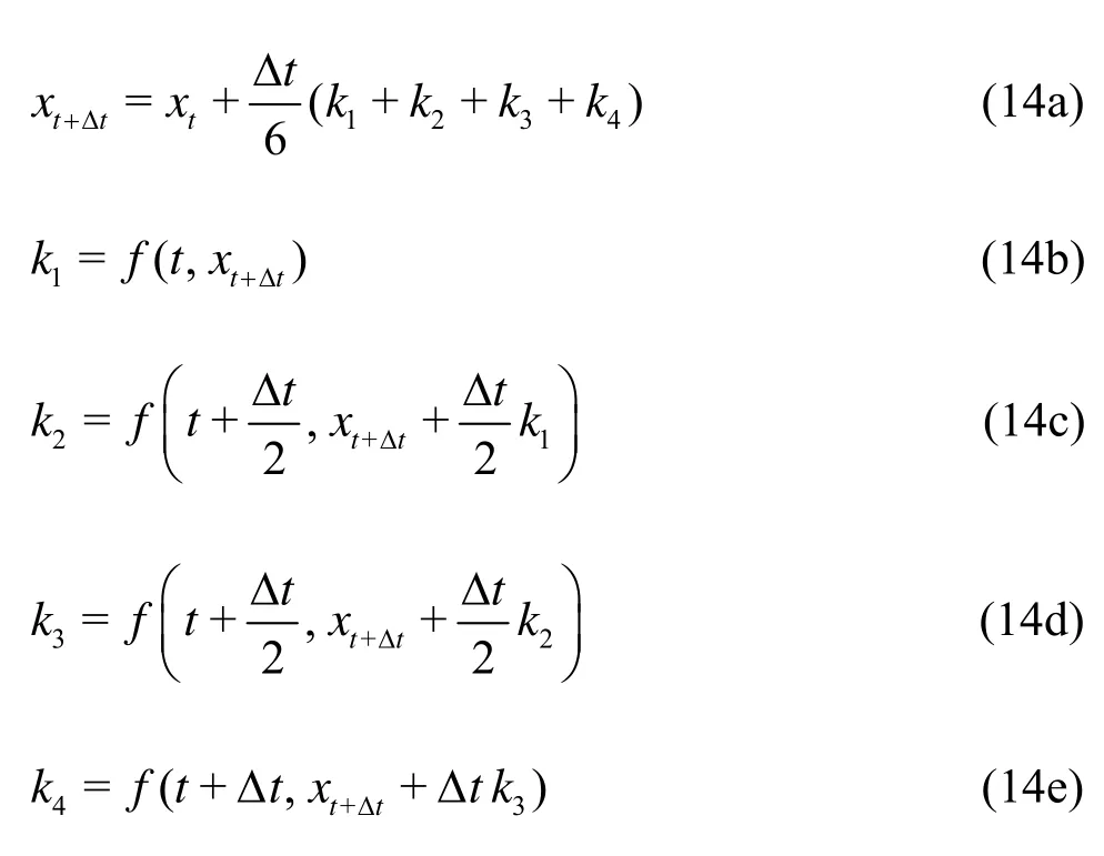
This method is called the 4th order implicit RK method, because all theki’s depend on unknown values ofxt+Δtnot yet calculated. Solving forxt+Δtat each time step requires an NR iterative procedure for the solution of the set of nonlinear equations. This can be achieved in the same manner as that shown in Table 2.

2. Mathematical programming based system identification

2.1Statement of the optimization problem

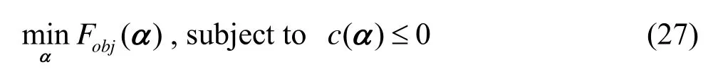
The optimization (or the mathematical programming problem) can be stated as follows[21]:

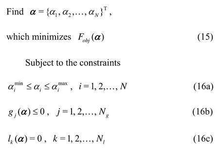
whereαis anN-dimensional vector called the design vector which contains the Design Variables (DV), in our case they are represented by the ship hydrodynamic coefficients to be determined, andFobj(α) is called the Objective Function (OF), andgi(α) andlk(α) are known as inequality and equality constraints, respectively. The number of variablesNand the number of constraintsNgand/orNlneed not be related in any way. The problem formulated using the condition (15) and the constraints (16) is called a constrained optimization problem, which can be solved using different algorithms.

In this work, a single OF is used in the optimization problem in order to identify ship hydrodynamic coefficients. Therefore, for the turning circle manoeuvre for instance, the OF is chosen as

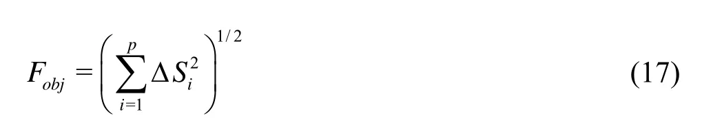
wherepis the number of sampling points, Δis the square root of the difference between the computed and the experimental ship positions on the trajectory, which depends on ship hydrodynamic coefficientsα.

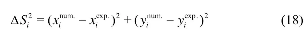
where the superscripts num. and exp. indicate the computed and experimental data respectively, and (xi,yi) are the coordinates of the pointi. For the case of a zigzag test, the expression ofFobjfollows

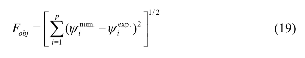
whereiψis the ship’s heading angle, which depends also on ship hydrodynamic coefficientsα,pis the number of sampling points where numerical solution has to be compared to the experimental measurements. The optimization problem stated in the condition (15) and the constraints (16) can be solved using different approaches. One of the most efficient approaches is related to the so-called mathematical programming techniques, where not only information on the OF are necessary but also values of the gradients of the OF (and the constraints) with respect to the vector of design parametersαare required to update the solution from one iteration to the other.

Among all optimization algorithms related to the MP techniques, the Sequential Quadratic Programming (SQP) algorithm[17]is a widely applicable in various optimization fields to solve constrained problems in engineering science. The Broyden-Fletcher-Goldfarb-Shanno (BFGS) algorithm[16]is a part of the family of quasi-Newton algorithms, which may be used for the unconstrained optimization problems.

2.2Normalization and sensitivity analysis

Normalization of DV plays an important role in the convergence of the optimization algorithm and in the quality of the optimal solution. It consists in a linear transformation of the original variablesαinto new transformed variables, which is given by

whereAandBare constant diagonal matrix and vector respectively. Generally, the most frequently used variables normalization uses the lower and upper bounds such as

The normalization of the objective function is easily accomplished by dividing the objective function at each iteration by(=/), whereis the value of the objective function at the first iteration. Caution is to be taken ifis very low (e.g., 1×10–6) which may affect the values of the gradients and cause instability of the optimization algorithm. Constraints may be normalized using the same procedure.

Once the normalization is applied, the gradients of the OF have to be adapted to the new set of design variables

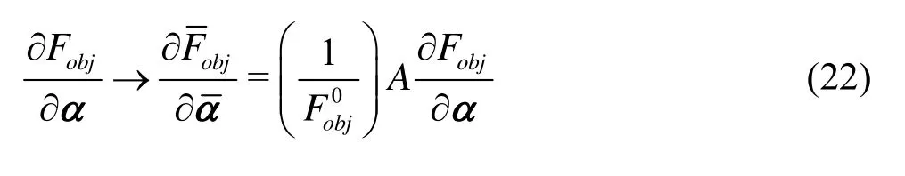
As was mentioned before, the optimization problem involving time-varying hydrodynamic coefficients is highly nonlinear, so the authors chose to proceed with the Finite Difference (FD) technique for the estimation of the gradients ?Fobj/?α

In the present investigationεwas fixed to 0.001.

2.3Brief recall of the BFGS method

Both the BFGS and SQP techniques belong to the Newton-like methods which are based on a quadratic approximation, more exactly in the secondorder Taylor approximation ofFobj(x) aboutα(k).

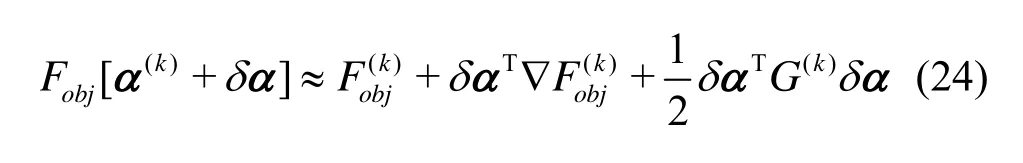
with ?the gradient vector andG(k)the Hessian tensor of the OF at iterationk. The stationary point of this approximation is a solution of a linear system of equations

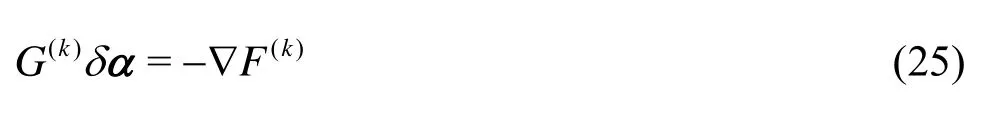
It is unique if(k)Gis non-singular and corresponds to a minimum if(k)Gis positive definite. In the BFGS method(k)

Gare approximated by the symmetric matrices(k)

H, which are updated from iteration to iteration using the most recently obtained information. By considering=?-?, the BFGS updating formula is given by[20]

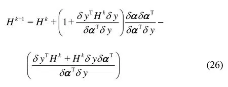
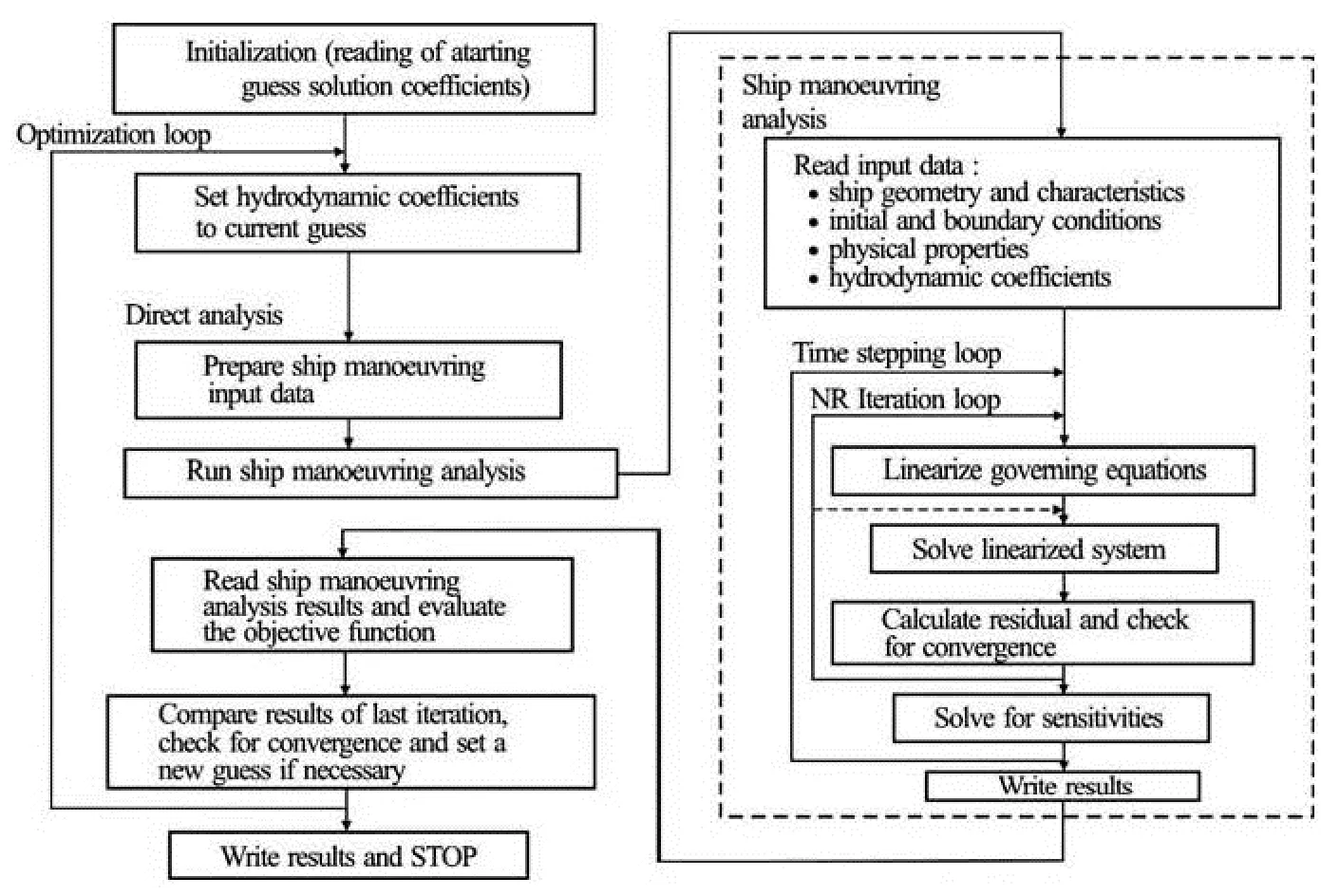
Fig.4 Flowchart of the optimization procedure for the identification of hydrodynamic coefficients

Global convergence has been proved for the BFGS method with inexact line searches, applied to a convex objective function[16]. The BFGS method with inexact line searches converges linearly if(k)Gis positive definite. The contemporary optimization literature[19]suggests the BFGS method is a preferable choice for general unconstrained optimization based on a line search prototype algorithm.

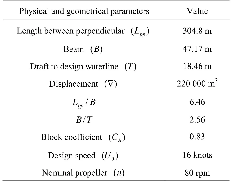
Table 3 Parameters of the ESSO 190 000-dwt oil tanker[7]

2.4Brief recall of the SQP method

The SQP algorithm belongs to the so-called constrained optimization methods, which are much more complex to formulate[17]. Many algorithms for their solution are based on transformation of the constrained problem to a sequence of unconstrained optimization subproblems whose solutions converge to the solution of the constrained problem. For instance, for a typical constrained optimization problem given by the condition (15) and the constraints (16), it can be written in a more general form

whereα,Fobjare already defined andcrepresents the nonlinear constraints (gi(α),lk(α) in formula (22)). Using the Lagrangian functionLa(α,λ)=Fobj(α)+λTc(α) one can derive first and higher order optima- lity conditions.

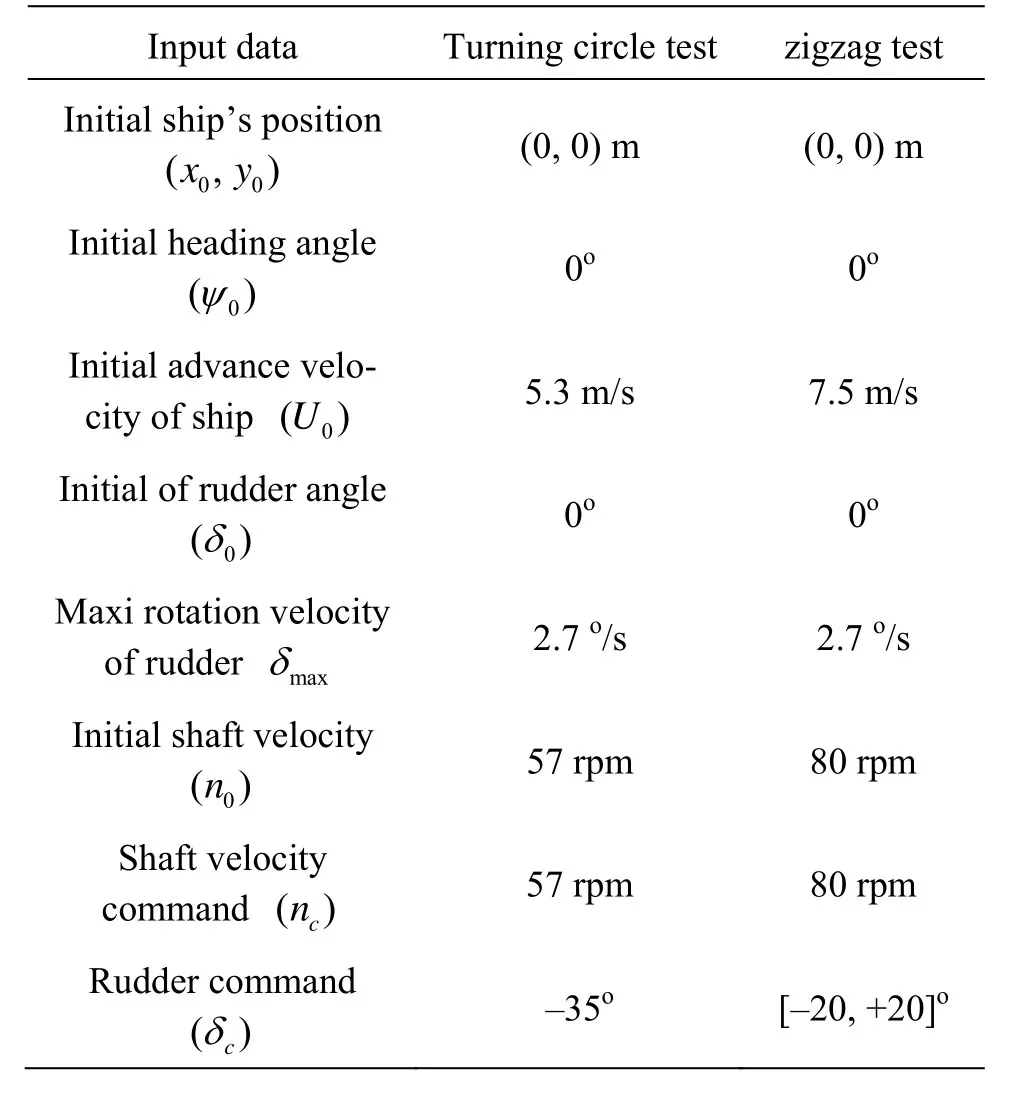
Table 4 Input data for turning circle and zigzag (ESSO 190 000-dwt oil tanker model)

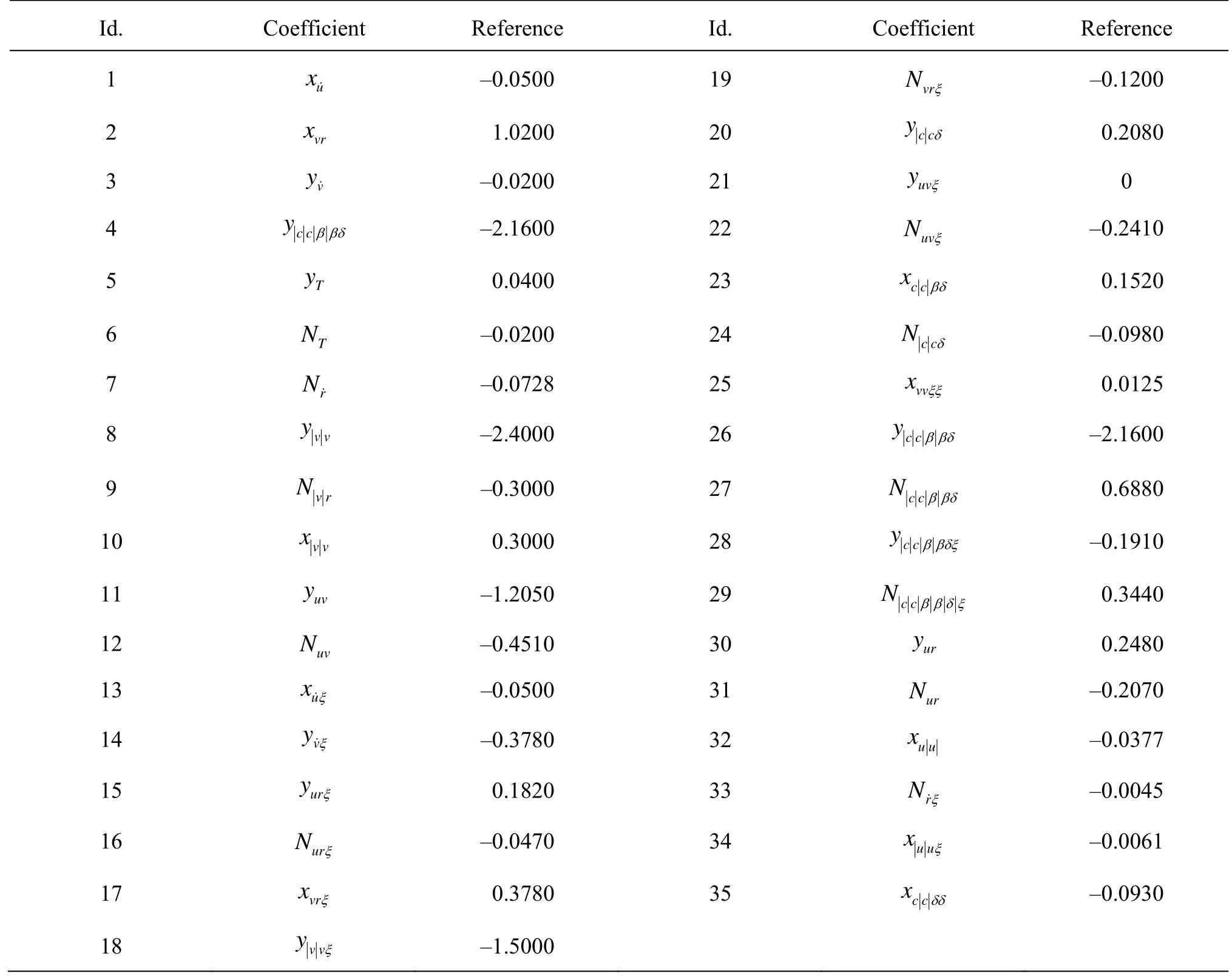
Table 5 Reference hydrodynamic coefficients of the ESSO 1190 000-dwt oil tanker model

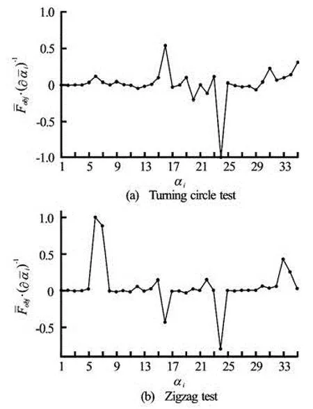
Fig.5 Sensitivity analysis

We note that all vectors and matrices depend on the optimization variablesαor the Lagrange multipliersλor both. For clarity, we suppress this dependence.

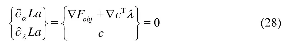
This expression represents a system of nonlinear equations, and the Jacobian of this system of equations is called the Karush-Kuhn-Tucker (KKT) matrix of the optimization problem. A Newton step on the optimality conditions is given by

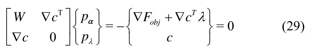
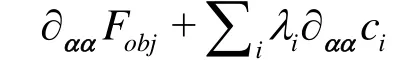
Table 6 Most sensitive coefficients of the ESSO 190 000-dwt oil tanker model

Finally, the proposed numerical procedure for the identification of hydrodynamic coefficients based on MP techniques can be summarized into three main steps:

(1) Calculate the ship trajectory with original coefficientsαfrom dynamic ship motion equations given by (8).

(2) Filter the most sensitive coefficientsSαamong all othersα, based on the sensitivity analysis.

(3) Calculate optimal valuesαoptfor only sensitive coefficientsSα, by carrying out the optimization procedure using SQP or BFGS algorithms.

The flowchart of the optimization procedure is shown in Fig.4.

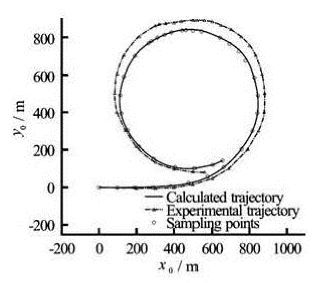
Fig.6 Ship trajectory using initial reference hydrodynamic coefficients

3. Numerical applications, results and discussion

The proposed procedure has been validated through turning circle and zigzag manoeuvres accordingly to the IMO and based on experimental data of sea trials of the ESSO 190 000-dwt oil tanker[7]. The associated physical and geometrical parameters related to the ship are given in Table 3.

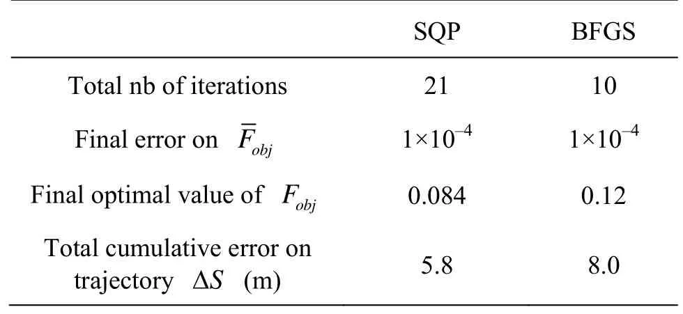
Table 7 Summary of final optimal solutions obtained by both SQP and BFGS in turning circle test

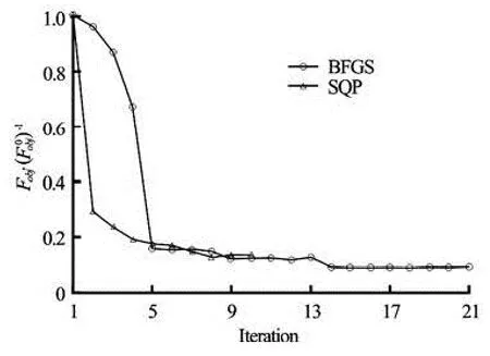
Fig.7 Evolution of the OF during the optimization process in turning circle manoeuvre

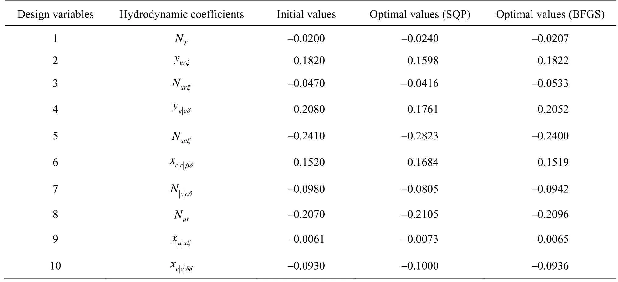
Table 8 Optimal hydrodynamic coefficients in turning circle test

The associated input data related to the turning circle test and to the zigzag manoeuvre are presented in Table 4.

In the present application, it is found that 35 hydrodynamic coefficients are necessary to control the manoeuvrability of the ESSO 190 000-dwt oil tanker model[7]. Thus, these coefficients (see Table 5) are used as as initial guess for the numerical processing.

The numerical identification procedure starts from original reference values of all hydrodynamic coefficients ()αin the dynamic ship motion equations given in Eq.(8), which will be firstly analyzed through a sensitivity analysis procedure to select the most important parameters.

The sensitivity analysis will show how important is the relative gradient value ofFobjresponse for a small variation of the hydrodynamic coefficientiα. The gradient ofFobjat coefficientiαis computed using formula (23) and formula (24). This analysis consists of filtering the largest gradient corresponding to eachiα, which is accomplished using the following criteria

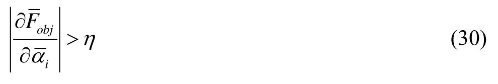
whereη=0.1 andis the normalized gradient value, which corresponds to the largest value of the gradient ?Fobj. By using the developed manoeuvring model, the sensitivities are computed and filtered using the above criterion. Variations of gradients are shown in Fig.5 for the turning circle and zigzag manoeuvres. As we can observe from Fig.5, only certain coefficients are of a great sensitivity (greater than 10%), and these sensitive hydrodynamic coefficients are identified and summarized in Table 6. We can also see that only 6 coefficients are common for the two turning circle and zigzag manoeuvres, this indicates that it is important to include the physical knowledge of the hydrodynamic problem in the identification process in order to insure a good result.

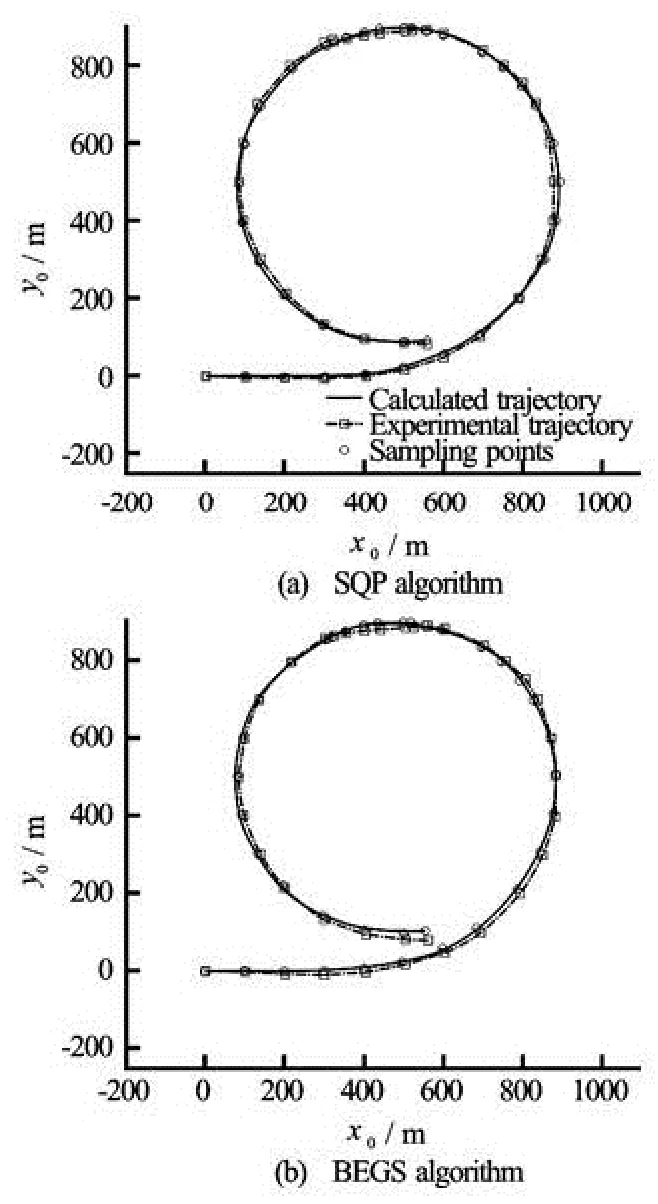
Fig.8 Comparison of ship trajectories after optimization

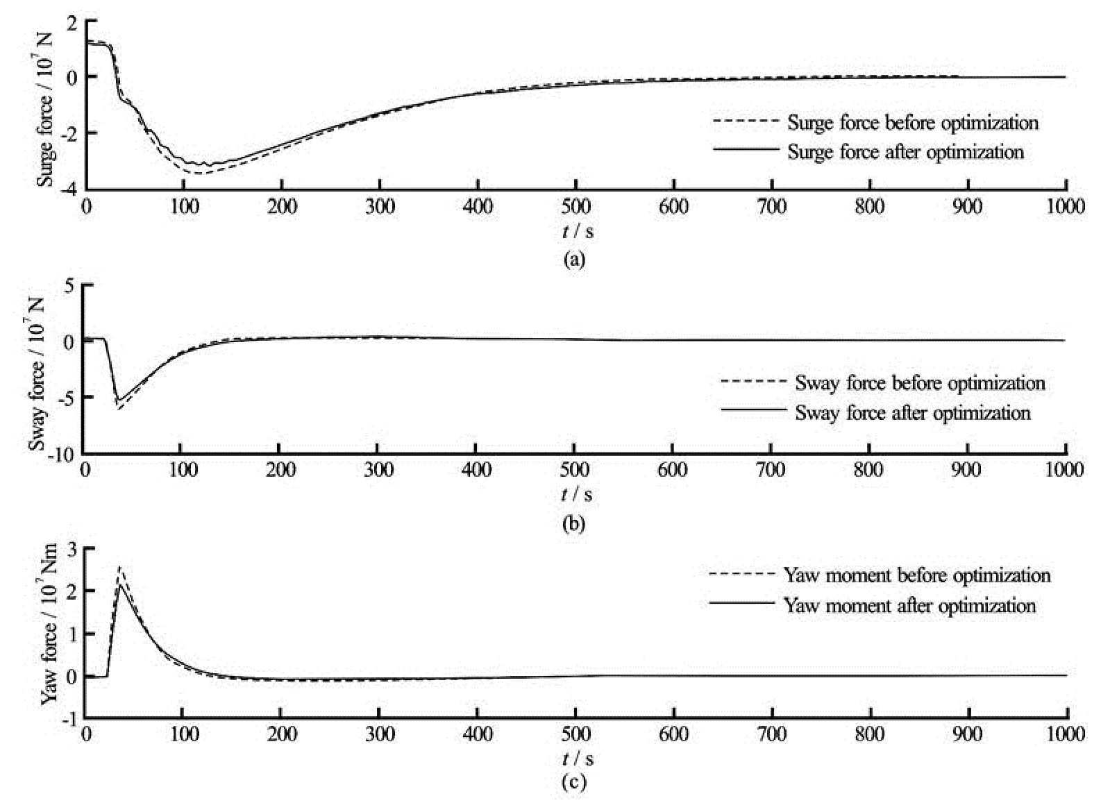
Fig.9 Comparison of hydrodynamic forces before and after optimization (SQP algorithm)

3.1Identification of hydrodynamic coefficients using a turning circle test

The proposed procedure has been validated using a turning circle test. For this purpose, we define an OF given by Eq.(17). This OF is considered to be sufficient for the case of a turning circle test, since no big variations arise in the ship dynamic motion.

At first the initial reference values of hydrodynamic coefficients are used and the developed ship manoeuvring model is used to evaluate the predicted trajectory. Figure 6 shows the calculated ship trajectory using our manoeuvring model. It is interesting to notice that before optimization, i.e., when starting with the initial reference values of hydrodynamic coefficients[19], the total cumulative error on the ship trajectory was ΔS=68 m.

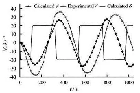
Fig.10 Comparison of the heading angle using initial reference hydrodynamic coefficients

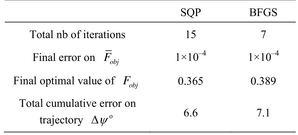
Table 9 Summary of final optimal solutions obtained by both SQP and BFGS in zigzag test

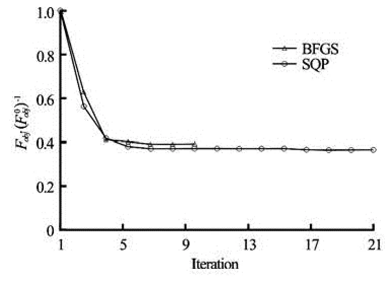
Fig.11 OF evolution during the optimization process in the zigzag manoeuvre

We definep=40 as the total number of experimental sampling points in the Eq.(17). The identification procedure has been carried out by using SQP andBFGS algorithms with a convergence criterion based on the error on the OF as 1×10–4and a maximum number of iterations of 50. Convergence has been achieved in 21 iterations for the SQP algorithm with a final optimal OF relative value of 0.084 and only in 10 iterations for the BFGS algorithm with a final optimal relative value of the OF of 0.12. A summary of final optimal solutions obtained by both the SQP and BFGS algorithms is given in Table 7.

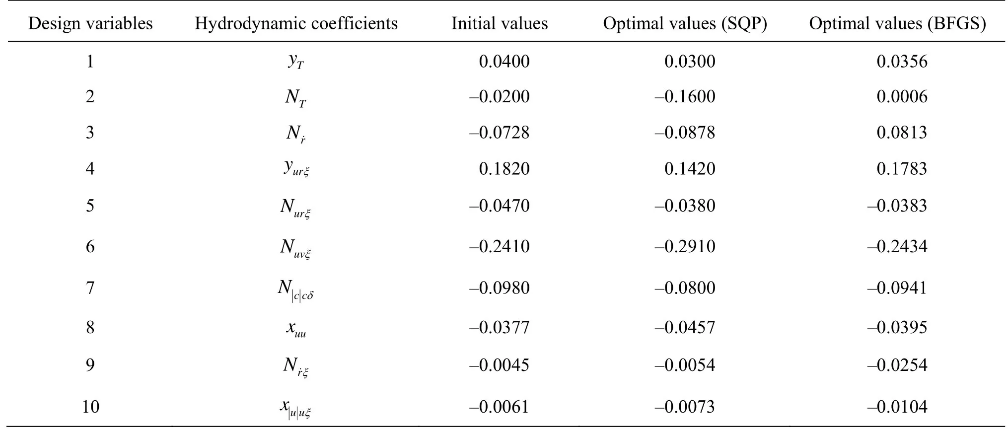
Table 10 Optimal hydrodynamic coefficients in zigzag tes

Figure 7 shows the evolution of the OF for both the SQP and BFGS algorithms during the optimization process. We can observe clearly the good convergence of both algorithms, which is mainly due to the normalization procedure affected to the DV and to the OF. We can notice also that the BFGS algorithm is faster than the SQP algorithm, which is already predictable since the first algorithm does not take into account the nonlinear constraints in the optimization process.

From Table 7, we can see that the SQP algorithm is more accurat than the BFGS algorithm because it leads to a minimal cumulative error for the trajectory of 5.8 m only. The optimal hydrodynamic coefficients obtained at the end of the optimization process are summarized in Table 8.

Figure 8 shows the optimal solutions obtained at the end of the optimization process. We can observe that both the SQP and BFGS algorithms predict correctly the experimental ship trajectory. A detailed comparison of the obtained trajectories shows that the result obtained using the SQP algorithm is more accurate than the BFGS one, since the total cumulative error between the experimental trajectory and the predicted one is very small relatively compared to the length of the ESSO 190 000-dwt oil tanker.

Figure 9 shows the evolutions of the surge and the sway forces as well as the yaw moment before and

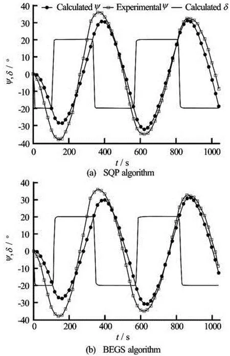
Fig.12 OF comparison of the heading angle after optimization (BFGS algorithms)

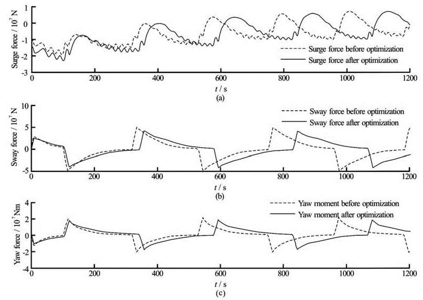
Fig.13 OF Comparison of hydrodynamic forces before and after optimization (SQP algorithm)

after optimization using the SQP algorithm. From Fig.9 it appears that at the beginning of turning circle test on the port side of the ship, absolute values of the hydrodynamic forces are reduced, therefore the gyration radius of the predicted trajectory obtained after optimization is larger than the gyration radius of the initial trajectory. We can explain this phenomenon by comparing the values of the hydrodynamic coefficients before and after using the SQP method directly from Table 7. At first, among all components of surge forces,xccδδappears to be the most important component because this component acts on the rudder surface axis when the rudder rotates.xccδδincreases from –0.093 to –0.1, which means that the resistance of rudder inxaxis is increased, and therefore the ship turns more difficultly towards the port side. We can observe also from Table 7 thatyccδis the most important component which acts on the rudder surface in theyaxis. Thenyccδis reduced from 0.208 to 0.1761, which means that the ship turns more slowly towards the port side. Finally, we can remark from Table 7 thatNccδis the biggest component among all yaw moments, which is basically caused by rudder forces when the last rotates. ThenNccδis reduced from –0.098 to –0.0805, which indicates that the yaw moment is reducing when the ship turned towards the port side.

3.2Identification of hydrodynamic coefficients using a zigzag test

The second application used to show the efficiency of the proposed procedure is a zigzag test. In this case, we define an OF based on the Eq.(19). The OF Eq.(17) used in the turning circle test cannot be used in the present application because in the zigzag test there will be large variations in the heading angle during the dynamic ship motion. As in the previous case, at first the initial reference values of hydrodynamic coefficients, given in Table 5, are used in the developed ship manoeuvring model to evaluate the predicted heading angle. Figure 10 shows the calculated ship heading angle using our manoeuvring model. It is interesting to notice that before optimization, i.e., when starting with the initial reference values of hydrodynamic coefficients[18], the total cumulative error on the ship trajectory is Δψ=17.3o.

We define in this applicationp=53 as the total number of experimental sampling points in the Eq.(19). The identification procedure has been carried out by using the SQP and BFGS algorithms with a convergence criterion based on the error on the OF as 1×10–4and a maximum number of iterations of 50. Convergence has been achieved in 15 iterations for the SQP algorithm with a final optimal OF relative value of 0.365 and only in 7 iterations for the BFGS algorithm with a final optimal relative value of the OF of 0.389. A summary of the final optimal solutions obtained by both the SQP and BFGS algorithms is given in Table 9.

Figure 11 shows the evolution of the OF for both the SQP and BFGS algorithms during the optimization process.

We can observe clearly the good convergence of both algorithms, which is mainly due to the normalization procedure affected to the DV and to the OF. We can also notice that the BFGS algorithm is faster than the SQP algorithm, which is already predictable

since the first algorithm does not take into account the nonlinear constraints in the optimization process.

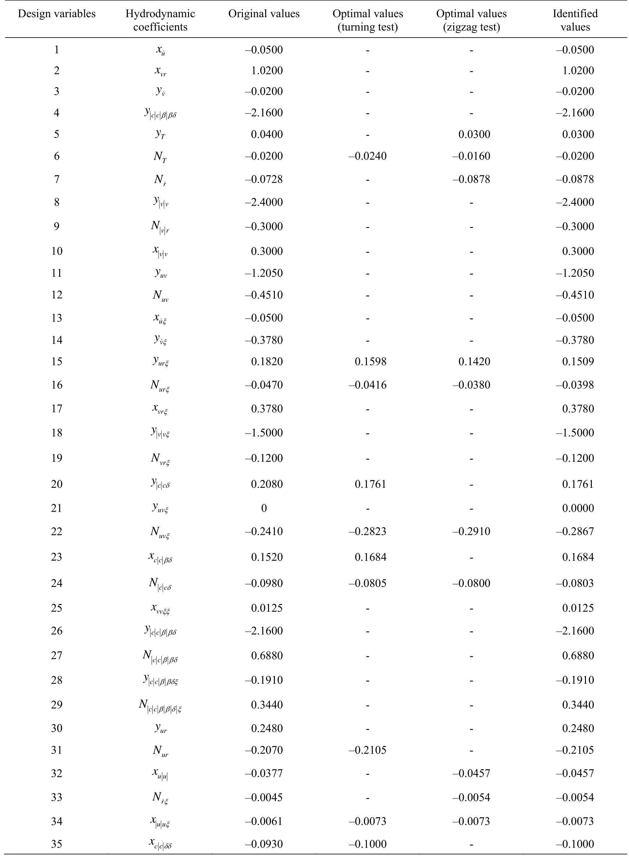
Table 11 Identified hydrodynamic coefficients for the ESSO 19 000-dwt oil tanker model

From Table 9, we can see that the SQP algorithm is more precise than the BFGS algorithm because it led to a minimal cumulative error on the heading angle of 6.6oonly. The optimal hydrodynamic coefficients obtained at the end of the optimization process are summarized in Table 10.

Figure 12 shows the optimal solutions obtained at the end of the optimization process. We can observe that both the SQP and BFGS algorithms predict correctly the experimental ship heading angle. A detailed comparison of the obtained heading angle shows that the result obtained using the SQP algorithm is more accurate than the BFGS one, since the total cumulative error between the experimental trajectory and the predicted one is very small relatively compared to the length of the ESSO 190 000-dwt oil tanker. Figure 13 shows the evolutions of the surge and the sway forces as well as the yaw moment before and after optimization using the SQP algorithm.

From the result of coefficient identification for turning circle and zigzag manoeuvres, we can choose finally a set of identified hydrodynamic coefficients for ESSO 190 000-dwt oil tanker model, which may be used for both two tests as well as for other manoeuvring simulations. This set has 35 hydrodynamic coefficients, which includes the mean optimal values of 6 shared most sensitive coefficients, the optimal values of 8 independent most sensitive coefficients of each test, and 21 other original coefficients that influence weakly the gradient of OF. For more details, we summarize all of coefficients before and after optimization in Table 10.

4. Conclusions

This investigation proposes, for the first time, a mathematical programming based on system identification for manoeuvring of large tankers that are governed by a well-established set of nonlinear equations of motion. The identification procedure is based on the coupling between ship manoeuvring simulation model and mathematical programming techniques by the use of the SQP and BFGS algorithms.

In the implemented manoeuvring model, the propulsion hydrodynamics, rudder hydrodynamics and manoeuvring hydrodynamics are strongly coupled. The model has been validated using experimental data of sea trials of the ESSO 190 000-dwt oil tanker model for the turning circle and zigzag manoeuvres, using 35 hydrodynamic coefficients. In the turning circle test, it is found that the SQP algorithm predicted accurately the experimental trajectories, with a total cumulative error on trajectory of 5.8 m, starting from an initial error of 69 m (before minimization). In the zigzag test of ship heading, the SQP algorithm gives a final cumulative error 6.6o, compared to the starting initial error of 17.3o. In the proposed mathematical programming based system identification, it is found that only 10 distinct hydrodynamic derivatives are identified to be sensitive in the turning circle and zig-zag manoeuvres respectively. With these known parameters, the proposed system identification technique obviates the need to know 25 other parameters. Finally, through the application of the ESSO 190 000-dwt oil tanker, we show that it is possible to use a combination of 14 hydrodynamic derivatives from both turning circle and zigzag manoeuvres, which may be used for both the turning circle, zig-zag tests and other manoeuvring simulations. Further developments of the presented procedure by introducing meta-modelling techniques based on response surfaces models and design of experiments are undertaken by the authors in order to assess the robustness and efficiency for a wider range of manoeuvring simulations.

Acknowledgements

The authors wish to thank the Vietnam Ministry of Education and Training, and the French Ministry of Ecology, Sustainable Development and Transport (CETMEF) for their financial support. They also would like to thank the anonymous reviewers for their helpful and useful comments to improve the manuscript.

[1] RAWSON K. J., TUPPER E. C. Basic ship theory[M]. Fifth Edition, Oxford, UK: Butterworth-Heinemann, 2001, 2: 368.

[2] HOCHBAUM A. C. Manoeuvring committee report and recommendations[C]. 25th International Towing Tank Conference. Fukuoka, Japan, 2008, 14-20.

[3] ARAKI M., SADAT-HOSSEINI H. and SANADA Y. et al. Estimating maneuvering coefficients using system identification methods with experimental, system-based, and CFD free-running trial data[J]. Ocean Engineering, 2012, 51: 63-84.

[4] JI Sheng Cheng, OUAHSINE Abdellatif and SMAOUI Hassan et al. 3-D numerical simulation of convoy-generated waves in a restricted waterway[J]. Journal of Hydrodynamics, 2012, 24(3): 420-429.

[5] FONFACH J. M. A., SUTULO S. and GUEDES SOARE C. Numerical study of ship-to-ship interaction forces on the basis of various flow models[C]. The Second International Conference on Ship Manoeuvring in Shallow and Confined Water. Trondheim, Norway, 2011.

[6] DAN O., RADOSLAV N. and LIVIU C. et al. Identification of hydrodynamic coefficients for manoeuvring simulation model of a fishing vessel[J]. Ocean Engineering, 2010, 37(8-9): 678-687.

[7] THE MANOEUVRING COMMITTEE. The final report and recommandations to the 24th ITTC[C]. Pro-ceeding of the 24th International Towing Tank Conference. Edinburgh, UK, 2005, 1: 137-198.

[8] SUTULO S., MOREIRA L. and SOARES C. G. Mathematical models for ship path prediction in manoeuvring simulation systems[J]. Ocean Engineering, 2002, 29(1): 1-19.

[9] NEVES M. A. S., RODRIGUEZ C. A. A coupled nonlinear mathematical model of parametric resonance of ships in head seas[J]. Applied Mathematical Modelling, 2009, 33(6): 2630-2645.

[10] YOSHIMURA Y. Mathematical model for manoeuvring ship motion[C]. Workshop on Mathematical Models for Operations involving Ship-Ship Interaction. Tokyo, Japon, 2005.

[11] YOON H. K., RHEE K. P. Identification of hydrodynamic coefficients in ship manoeuvring equations of motion by Estimation-Before-Modeling technique[J]. Ocean Engineering, 2003, 30(18): 2379-2404.

[12] VIVIANI M., BONVINO C. P. and DEPASCALE R. et al. Identification of hydrodynamic coefficients from standard manoeuvres for a series of twin-screw ships[C]. 2nd International Conference on Marine Research and Transportation. Naples, Italy, 2007, 99-108.

[13] RAJESH G., BHATTACHARYYA S. K. System identification for nonlinear manoeuvring of large tankers using artificial neural network[J]. Applied Ocean Research, 2008, 30(4): 256-263.

[14] SEO M. G., KIM Y. Numerical analysis on ship manoeuvring coupled with ship motion in waves[J]. Ocean Engineering, 2011, 38(17-18): 1934-1945.

[15] ZHANG Xin-guang, ZOU Zao-jian. Identification of Abkowitz model for ship manoeuvring motion usingε-support vector regression[J]. Journal of Hydrodynamics, 2011, 23(3): 353-360.

[16] DAI Y. H. Convergence properties of the BFGS algorithm[J]. Society for Industrial and Applied Mathematics, 2002, 13(3): 693-701.

[17] ZHANG J., ZHANG X. A robust SQP method for optimization with inequality constraints[J]. Computational Mathematics, 2003, 21(2): 247-256.

[18] OUAHSINE A., SERGENT P. and HADJI S. Modelling of non-linear waves by an extended Boussinesq model[J]. Journal of Engineering Applications of Comput Fluid Mechanics, 2008, 2: 11-21.

[19] TRAN K. T. Simulation and identification of hydrodynamic parameters for a freely manoeuvring ships[D]. Doctoral Thesis, Compiěgne, France: University of Technology of Compiègne, 2012.

[20] KAIDI S., ROUAINIA M. and OUAHSINE A. Stability of breakwaters under hydrodynamic loading using a coupled DDA/FEM approach[J]. Ocean Engineering, 2012, 55: 62-70.

[21] SOULI M., ZOLESIO J. P. and OUAHSINE A. Shape optimization for non-smooth geometry in two dimensions[J]. Computer Method in Applied Mechanics Engineering, 2000, 188(1-3): 109-119.

10.1016/S1001-6058(13)60426-6

* Biography: TRAN KHANH Toan (1979-), Male, Ph. D.

OUAHSINE Abdellatif,

E-mail: ouahsine@utc.fr