Dealing with the Data Imbalance Problem in Pulsar Candidate Sifting Based on Feature Selection

Haitao Lin and Xiangru Li

1 School of Mathematics and Statistics, Hanshan Normal University, Chaozhou 521000, China

2 School of Computer Science, South China Normal University, Guangzhou 510631, China; xiangru.li@gmail.com

Abstract Pulsar detection has become an active research topic in radio astronomy recently.One of the essential procedures for pulsar detection is pulsar candidate sifting (PCS), a procedure for identifying potential pulsar signals in a survey.However, pulsar candidates are always class-imbalanced, as most candidates are non-pulsars such as RFI and only a tiny part of them are from real pulsars.Class imbalance can greatly affect the performance of machine learning (ML) models, resulting in a heavy cost as some real pulsars are misjudged.To deal with the problem,techniques of choosing relevant features to discriminate pulsars from non-pulsars are focused on,which is known as feature selection.Feature selection is a process of selecting a subset of the most relevant features from a feature pool.The distinguishing features between pulsars and non-pulsars can significantly improve the performance of the classifier even if the data are highly imbalanced.In this work,an algorithm for feature selection called the K-fold Relief-Greedy(KFRG)algorithm is designed.KFRG is a two-stage algorithm.In the first stage,it filters out some irrelevant features according to their K-fold Relief scores, while in the second stage, it removes the redundant features and selects the most relevant features by a forward greedy search strategy.Experiments on the data set of the High Time Resolution Universe survey verified that ML models based on KFRG are capable of PCS,correctly separating pulsars from non-pulsars even if the candidates are highly class-imbalanced.

Key words: methods: data analysis – (stars:) pulsars: general – methods: statistical

1.Introduction

Pulsars are highly magnetized, rotating, compact stars that emit beams of electromagnetic radiation out of their magnetic poles.They are observed as signals with short and regular rotation periods when their beams are received by the Earth.The study of pulsars is of great significance to promote the development of astronomy, astrophysics, general relativity and other fields.As a remarkable laboratory, they can be used for research on the detection of gravitational waves (Taylor 1994),observation of the interstellar medium (ISM; Han et al.2004),the conjecture of dark matter (Baghram et al.2011) and other research fields.Therefore, many pulsar surveys (projects) have been carried out or are ongoing to search for more new pulsars.These pulsar surveys have produced massive observation data in the form of pulsar candidates.For example,the number of pulsar candidates from the Parkes Multibeam Pulsar Survey (PMPS;Manchester et al.2001) is about 8 million; the High Time Resolution Universe (HRTU) pulsar survey (Keith et al.2010;Levin et al.2013) has returned 4.3 million candidates (Morello et al.2014);the LOFAR Tied-Array All-Sky Survey(LOTAAS;van Haarlem et al.2013)has accumulated 3 million candidates,etc.With the development of modern radio telescopes, such as the Five-hundred-meter Aperture Spherical radio Telescope(FAST;Nan 2006;Nan et al.2011,2016)and Square Kilometre Array(SKA;Smits et al.2009),the amount of pulsar candidates has increased exponentially.However, of this vast amount of candidates,only a small part of these candidates are real pulsars,while others are radio frequency interferences (RFIs) or other kinds of noises(Keith et al.2010).Thus,one essential process of pulsar search is to separate the real pulsar signals from nonpulsar ones, which is known as pulsar candidate sifting (PCS).

Recently, quite a few machine learning (ML) methods have been applied to PCS.They are mainly divided into two types according to their inputs—-models based on artificial features and models based on image-driven approaches.

Figure 1.Diagnostic plots and summary of statistical characteristics of a pulsar candidate.

Artificial features are designed in accordance with the different nature between pulsars and non-pulsars.These features were extracted by their physical background (we call empirical features)or statistical characteristics(statistical features)and can be clearly explained.Typically, Eatough et al.(2010) first extracted 12 empirical features from candidates as inputs of an Artificial Neural Network (ANN; Haykin 1994; Hastie et al.2005) model for PCS.The ANN model was experimented with in the PMPS survey (Manchester et al.2001) and achieved a recall rate of 93% (recall rate is a performance measure defined as a ratio between the number of successfully predicted pulsars and the total number of real pulsars).Moreover, Bates et al.(2012) constructed another ANN with 22 features as inputs in HTRU-Medlat(Keith et al.2010)and achieved a recall of 85%.To improve the performance of PCS, Morello et al.(2014)empirically designed six empirical features to build a model called Straightforward Pulsar Identification using Neural Networks(SPINN),which even achieved both a high recall of 100%and a low false positive rate (FPR).Then, a purpose-built treebased model called Gaussian Hellinger Very Fast Decision Tree(GHVFDT) (Lyon et al.2014) was applied to PCS with eight newly designed features.These features are statistics computed from both the folded profile and the dispersion measure (DM)searching curve (defined in Section 2.1).They are evaluated,using the joint mutual information criterion to help identify relevant features.Later, Tan et al.(2017) pointed out that the GHVFDT based on these eight features is insensitive to pulsars with wide integrated profiles.They therefore proposed eight other new features and built an ensemble classifier with five different decision trees(DTs)to improve the performance of the detection.

As for image-driven PCS models, they are based on deep learning networks,where deep features were extracted from their diagnostic plots (Figure 1).Zhu et al.(2014) first proposed the Pulsar Imaged-based Classification System(PICS),whose inputs are four mainly diagnostic plots, i.e., sub-integration, subband,folded signal and DM-curve(their definitions can be referred to in Section 2.1).Wang et al.(2019) then improved PICS and designed a PICS-ResNet model which is composed of two Residual Neural Networks (ResNets), two Support Vector Machines (SVMs) and one Logistic Regression (LR).Guo et al.(2019) used a combination of a deep convolutional generative adversarial network(DCGAN)and an SVM to apply to the HTRU Medlat and PMPS surveys.Then they constructed a model by combining the DCGAN and MLP neural networks trained with the pseudoinverse learning autoencoder (PILAE)algorithm, achieving excellent results on class-imbalanced data sets (Mahmoud & Guo 2021).Recently, Xiao-fei et al.(2021)designed a 14-layer deep residual network for PCS, using an oversampling technique to adjust the imbalance ratio(IR)of the training data.The experiments on HTRU achieved both a high precision and a 100% recall (Xiao-fei et al.2021).As far as intelligent identification is concerned, deep learning methods have shown great significant application in the PCS.More related works can be referred to in Guo et al.(2019),Zhang et al.(2019), Lin et al.(2020), Xiao et al.(2020), Zeng et al.(2020),Cai et al.(2023).Although these models showed an advantage in performance, they failed to quantify significant differences between pulsars and non-pulsars since the deep features extracted from them were inexplicable or incomprehensible.

One of the greatest challenges in ML is the class imbalance problem (Japkowicz et al.2000), where the distribution of instances with labels is skewed.In the case of a binary classification problem,class imbalance implies that the number of members in one class is far less than that in the other class in a data set.We refer to these two categories as the majority and the minority, respectively.The ratio between the total number of the majority and that of the minority is called IR.A machine classifier with high IR tends to judge an unknown item as a major class, resulting in low recall rates.For instance, the HTRU data set is a highly class-imbalanced set,as the number of non-pulsar signals is close to 90,000 while the number of pulsar signals is only 1196.To address the class imbalance problem,oversampling methods have been implemented before training.For instance, Morello et al.(2014) balanced their training set by random oversampling to a 4:1 ratio of nonpulsars to pulsars.Bethapudi et al.(Bethapudi & Desai 2018)and Devine et al.(2016)adopted the Synthetic Minority Oversampling Technique (SMOTE; Chawla et al.2002) to produce more positive samples and raise the recall of the models.SMOTE is one of the most commonly used oversampling methods to handle the imbalanced data distribution problem.It generates virtual instances by linear interpolation for the minority class.These instances are generated by randomly choosing one or more of the k-nearest neighbors for each example in the minority class.After the oversampling process,the data are reconstructed to be class-balanced.However,this is not reflective of the real problem faced and is an artifact of data processing since these generative instances are virtual, random and not from the real world.

In our work, instead of raising the performance of PCS models by balancing the training data of candidates,we improve the pulsar accuracy of the models in perspective of the feature representation, which is called feature selection or variable selection(Tang et al.2014)in ML terminology.More precisely,feature selection is the process of selecting a subset of relevant features from the feature candidate pool.Feature selection is necessary in the data preprocessing stage,as some of the features may be redundant or irrelevant.These redundant or irrelevant features will decrease the performance of the sifting model.A well-designed feature selection algorithm will significantly improve the predictive ability of the ML sifting model.For the above considerations, an algorithm of feature selection called K-fold Relief-Greedy (KFRG) is proposed in this work.KFRG is a purpose-built two-stage algorithm: the first stage is to filter out some irrelevant features from the candidate features by Relief score,while the second stage is to select the most relevant features in a greedy way.To verify the effectiveness of KFRG for PCS, several typical ML classifiers are evaluated, including C4.5 (Quinlan 2014), Adaboost (Freund & Schapire 1997),Gradient Boosting Classification (GBC; M?ller et al.2016),eXtreme Gradient boosting (XGboost; Chen & Guestrin 2016),etc.Our experiments were performed on the public data of HTRU (Keith et al.2010).

The article is arranged as follows.Section 2 gives a description of the HTRU dateset as well as some related works.In Section 3, as many as 22 artificial features are introduced,including six empirical features from Morello et al.(2014),eight statistical features designed by Lyon et al.(2016)and eight additional statistical features proposed by Tan et al.(2017).These features are collected to be examined in the next study.In Section 4,KFRG as an algorithm of feature selection for PCS is proposed.Experiments based on KFRG are carried out on HTRU survey data in Section 5,and the discussion and conclusion are presented in Section 6.

2.Data and Preliminary Works

2.1.Pulsar Candidates and the HTRU Data Set

A pulsar candidate is originally a piece of signal from the receiver of a radio telescope during the observation time.Most commonly, it is processed by PulsaR Exploration and Search TOolkit (PRESTO; Ransom 2001), a typical software for pulsar search and analysis.Then the candidate is represented using a series of physical values and a series of diagnostic plots as Figure 1 shows.On the left,the plots from top to bottom are:a subband plot,a sub-integration plot and a folded profile of the signal.A subband plot displays the pulse in different bands of observed frequencies;a sub-integration plot shows the pulse in the time domain; a folded profile is the folded signal of its subbands by frequency or the folded signal of its subintegrations by period.On the right are two plots.One is a grid searching plot for DM and period.The other is a DMsearching curve.It is known that DM measures the number of electrons which a pulsar’s signal travels through from the source to the Earth.However, a real DM is unknown and should be obtained by trials.Then a grid searching plot on the right top of Figure 1 records the change of signal-to-noise ratio(S/N) as the trial DMs and the trial periods vary.A DM searching curve on the right middle describes the relationship between trial DM and its corresponding S/N, and the peak of the curve implies the most likely value of DM.

Our work is conducted on the HTRU survey.The HTRU data set is observed with two observatories, the Parkes radio telescope in Australia and the Effelsberg 7-beam system in Germany.HTRU is an ambitious(6000 hr)project to search for pulsars and fast transients in the entire sky, which is split into three areas: Low-latitude (covers±3°.5), Mid-latitude (Medlat;covers±15°) and High-latitude (covers the remaining sky<10°).The pipeline searched for pulsar signals with DMs from 0 to 400 pc·cm-3(DM is often quoted in the units of pc·cm-3,which makes it easy to estimate the distance between a given pulsar and the Earth),and also performed an accelerated search between -50 to +50 m s-2.

The HTRU data set was publicly released by Morello et al.(2014) and is available online3http://astronomy.swin.edu.au/～vmorello/.It consists of 1196 real pulsar candidates and 89,995 non-pulsars, which are highly classimbalanced, as only a tiny fraction of the candidates are from real pulsar signals (Table 1).

2.2.Machine Learning Classifiers

PCS can be described as a binary supervised classification issue in ML.Supervised learning(Mitchell et al.1997)is an ML task of learning a function that maps instances to their labels.Particularly, a classifier of PCS aims to learn function mapping features of the pulsar candidates to their categories—-pulsar or non-pulsar.To evaluate the effectiveness of selected features,the performance of classifiers should be estimated.

In our work, feature selection algorithms are evaluated by seven classifiers.Among them, DT (Quinlan 2014), LR(Hosmer et al.2013)and SVM(Suykens&Vandewalle 1999)are normal classifiers, while Adaptive boosting (Adaboost;Freund &Schapire 1997),GBC (M?ller et al.2016),XGboost(Chen & Guestrin 2016) and Random Forest (RF; Liaw et al.2002)are ensemble learning classifiers.The principles of these classifiers are different and representative.For example, a typical DT classifier is based on the information gain ratio while SVM tries to find the best hyperplane which represents the largest separation between the two classes.Ensemble methods (Dietterich et al.2002) use multiple weak classifiers such as DT to obtain a strong classifier.Interested readers can refer to their references for details(Mitchell et al.1997;Mohri et al.2018).

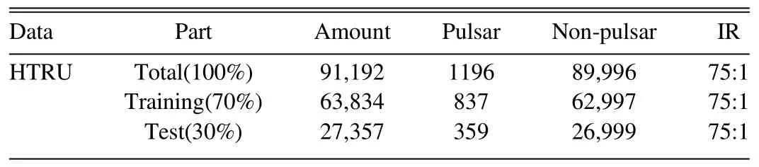
Table 1 The Description of our Experimental Data

2.3.Performance Metric

To evaluate the performance of a classifier on classimbalanced data, typically on pulsar candidate data, four most relevant metrics are given.They are the Recall rate, Precision rate, F1score and FPR.They can be expressed by True Positives (TP), True Negatives (TN), False Positives (FP) and False Negatives (FN).

In binary classification, recall, defined by TP/(TP+FN),where TP denotes the amount of true pulsars predicted and TP+FN the total amount of true pulsars.It measures how many pulsars could be correctly predicted pulsars from all the real pulsars.Precision, defined by TP/(TP+FP), measures how many true pulsars would be predicted correctly out of the candidate prediction tasks.However, recall and precision compose a relationship that opposes to each other, as it is probable to increase one at the cost of reducing the other.Therefore,F1score,defined as the harmonic mean of recall and precision, i.e., (2·Precision·Recall)/(Precision+Recall), is a trade-off between them.As for FPR, it measures the ratio of mislabelled non-pulsars out of all the non-pulsar candidates by FP/(TN+FP).It can be inferred by recall and precision.Therefore,we just need to focus on the recall,precision and F1score of a classifier.

3.Feature Pool

Before feature selection,a set of candidate features should be collected to be further selected, which is called a feature pool.The feature selection algorithm will be implemented on this pool to output a feature subset that has better representation.Considering that some of the candidate features are trivial for PCS, several guidelines for a feature pool were discussed in this section.

3.1.Guidelines of Candidate Features

To extract some robust and useful features, guidelines of feature design were proposed by PCS researchers.Morello et al.(2014) gave several suggestions, such as “ensuring complete robustness to noisy data”in order to“exploit properly in the low-S/N regime,”and“l(fā)imiting the number of features”to deny“the curse of dimensions.”Lyon et al.(2016)suggested that features should be designed to maximize the separation between positive and negative candidates, reducing the impact of class imbalance.

Based on suggestions from Morello et al.(2014) and Lyon et al.(2016),guidelines for candidate features in a feature pool were summarized as follows.Candidate features:

1.Should be distinguishable enough between pulsars and non-pulsars.A distinguishable feature will greatly improve the performance of the classifier.

2.Should be diversified.Considering the diversity of the feature source, both empirical features and statistical features should be included in the feature pool.

3.Should fully cover the space.Features should be extracted from the mainly diagnostic images, especially the sub-integration plot, the subband plot, the folded profile and the DM searching curve.

4.Can be easily extracted and calculated.

5.Should be controlled in a moderate total number.If the total number is small, some relevant features may be missed;if it is large,it will enlarge the computing cost of the feature selection algorithms.

3.2.Candidate Features in our Work

Following the guidelines in Section 3.1, 22 features have been collected (Table 2), which are candidate features from Morello et al.(2014),Lyon et al.(2016)and Tan et al.(2017).Among them,six features were defined by Morello et al.(2014)to build the SPINN model, eight statistical features were proposed by Lyon et al.(2016)as inputs to GHVFDT and eight additional features were introduced by Tan et al.(2017) to develop an ensemble classifier comprised of five different DTs.Details of these features are described in Table 2.

To demonstrate the discriminating capabilities of these features, one statistical approach is to show the distributions of pulsars and non-pulsars from each feature by box plots, which can graphically demonstrate the locality, spread and skewness groups of the features.Figure 2 displays box plots of our candidate features on HTRU.There are two box plots per feature.The red boxes describe the feature distribution for known pulsars,while the white ones are for non-pulsars mainlyconsisting of RFI.Note that the data of each feature were scaled by z-score, with mean zero and standard deviation one.The resulting z-score measures the number of standard deviations that a given data point is from the mean.Generally,the less the overlap of the red box and white box in a feature,the better the separability of the feature.However, the usefulness of features according to their box plots is only on a visual level.Measurable investigation of these features will be given in the next section.

Table 2 Notations and Definitions of 22 Candidate Features in Our Work

4.Feature Selection Algorithms

4.1.Motivation

A feature selection algorithm is a search technique for a feature subset from a feature pool.Irrelevant or redundant features not only decrease the calculation efficiency of ML models but also negatively affect their performances.Better selected features can be helpful when facing a data-imbalanced problem as described by Wasikowski & Chen (2010), and some practical algorithms have been proposed for a two-class imbalanced data problem(Yin et al.2013; Maldonado et al.2014).

There are main three categories of feature selection algorithms:filters, wrappers and embedded methods.Filter methods use a proxy measure to score a feature subset.Commonly,they include the mutual information (Shannon 1948), the point-biserial correlation coefficient (Gupta 1960) and Relief (Urbanowicz et al.2018)score.Wrapper methods score feature subsets using a predictive model.Common methods include grid search, greedy(Black 2012) and recursive feature elimination (Kira &Rendell 1992).An embedded feature selection method is an ML algorithm that returns a model using a limited number of features.

Our proposed algorithm of feature selection will combine the idea of a filter called Relief with a wrapper method named Greedy.On one hand, PCS, as a mission of binary supervised classification, is highly dependent on the constructive features between pulsars and non-pulsars.Thus, methods of filtering are preferably considered as they measure the relation between features and labels.In fact,measures by filters are able to capture the usefulness of the feature subset only based on the data,which are independent of any classifier.A Relief algorithm is one of the best measures of filters when compared with other filter methods.It weights features and avoids the problem of high computational cost in a combinatorial search.Thus, our proposed approach of feature selection for PCS is a Reliefbased algorithm.On the other hand, the selected features according to their Relief scores may be redundant.They involve more than two features with high Relief scores but they are strongly correlated,since one relevant feature may be redundant in the presence of another relevant feature (Guyon &Elisseeff 2003).To remove these redundant features, it follows the evolution of Relief scores to implement a Greedy technique.

However, Greedy or Relief for feature selection has some shortcomings.Although Relief score is able to filter out some irrelevant features, it could not detect the redundant ones,which implies that if two features share the same information in terms of correlation measure, both of them are very likely judged as relevant or irrelevant.As for Greedy, it can be utilized to reduce the number of features.Its computational cost increases in a quadratic way as the number of features increases, which makes the computation unaffordable.

Based on the considerations above, we combine Relief with the Greedy algorithm to propose a KFRG algorithm of feature selection for PCS.In the first stage,it filters out some irrelevant features according to their Relief scores, while in the second stage, it removes the redundant features and selects the most relevant features by a forward Greedy search strategy.Experimental investigations on HTRU showed that it improved the performance of most classifiers and achieved high both recall rate and precision (Section 5).

4.2.Relief Algorithm

Relief (Kira & Rendell 1992) is a filter algorithm of feature selection which is notably sensitive to feature interactions.It calculates a feature score for each feature which can then be applied to rank and select top scoring features for feature selection.Alternatively, these scores may be applied as feature weights to guide downstream modeling.Relief is able to detectconditional dependencies between features and their labels(pulsars and non-pulsars) and provide a unified view on the feature estimation in regression and classification.It is described as Formula (1).The greater the Relief score of a feature is, the more distinguishable the feature is, and corresponding features are more likely to be selected.

Figure 2.Box plots of features on HTRU.For each feature there are two distinct box plots, of which the red box describes the distribution for known pulsars in the feature, while the white one is for non-pulsars.

Algorithm 1.Relief Algorithm

Input:D; #Training data set S; #Features pool δ0; #A preset threshold Output:Δ.Set of selected features 1:Δ =[]# Initialization of the chosen features 2: for j 1: ∣S∣= do 3: Compute jδ by Equation (1)4: if j 0 δ>δthen 5: ∪{j }Δ = Δ 6: return Δ

4.3.Greedy Algorithm

A greedy algorithm is an algorithm that follows the problemsolving heuristic of making the locally optimal choice at each stage (Black 2012).The greedy strategy does not usually produce an optimal solution.Nonetheless, a greedy heuristic method may yield a locally optimal solution that approximates the global optimal solution in a reasonable amount of time.

In our algorithm, the objective function (target) is to maximize the F1score of a classifier, and thus our greedy implementation is designed to choose the best feature step by step from the rest of the feature pool.Here, “the best feature candidate” is the feature which contributes best to increase of the F1score of the classifier.Accordingly, the stopping criterion of our greedy implementation in the iteration procedures is that the F1score does not increase anymore, or the maximum number of selected features is more than a preset threshold Maxlen.

Maxlen is a hyperparameter to control the maximum number of selected features.On one hand, Maxlen should be large enough to enable as many candidate features as possible.A small Maxlen may miss some relative features and result in low performance.On the other hand, as Maxlen increases, so does the computational complexity (Goldreich 2008).Computational complexity is an important part of an algorithm design,as it gives useful information about the amount of resources required to run it.In fact, the computational complexity of Greedycanbeexpressed asO(Maxlen2)×O(L )according to Algorithm2,where the notationO(Maxlen2) means the run time or space requirements grow as the square of Maxlen grows,whileO(L ) represents the computational complexity of L which relies on both the choice of a classifier and the size of the input (feature).Thus, a large Maxlen implies a large computing cost.To evaluate a fit, Maxlen experiments with values ranging from 2 to 10 were carried out.Experimental investigation shows that as Maxlen increases, the average performance metrics improve rapidly at first,while they stay at a similar level when Maxlen is more than 8.The average recall and precision stay around 97.2% and 98.0% respectively for Maxlen larger than 8 as Table 5 affirms.Considering both the computational complexity and the performance, Maxlen is set to be 8.

Following the description above, our Greedy Algorithm of feature selection can be described as Algorithm 2.

Algorithm 2.Greedy Algorithm

Input:D; # Training data set S; # Features pool;L # Classifier Maxlen; # Maximum number of selected features Output:Sch.# Set of selected features 1:S ;ch =[] # Initialization of the chosen features 2:S S;un = # Initialization of the unchosen features 3: F 0;1= # Initialization value of F1 score 4: while S MaxLen∣ ∣< do 5: for j ?Sundo 6: S j ch L L( ∪{ })=# add j to a classifier 7: *j ch=?# choose the best feature 8: * *F F S j j argmaxj S 1 j un (L )F 1 1L ch( ( ∪{ })=9: if *F F 1> 1 10: *F F 1= 1 11: *S S j un un{ }=12: *S S j ch ch ∪{ }=# add j to a classifier 13: else 14: break 15: return Sch

4.4.KFRG Algorithm

Relief is easy to operate,but it is not very satisfying in some class-imbalanced scenarios, since it may underestimate those features with high discriminative ability that are in the minority, and ignores the sparse distributional property of minority class samples (Yuanyu et al.2019).That is, a feature with high Relief score pays more attention to the non-pulsars which are in the majority class and it is hard to identify the pulsars which are in the minority class and thus more promising pulsars will be missed.

To overcome these flaws,the K-fold Relief(KFR)algorithm was designed.The key improvement of KFR is to balance the data by recycling the minority and sampling from the majority.First,split the training data into minority samples and majority ones.Then, produce K disjoint subsets from the majority samples randomly, and merge each subset with the minority into K new data sets,each of which is relatively balanced with the same minority samples.Here,K is a preset integer which is normally the ratio of the majority classes to minority classes in the training data set.Finally, calculate the mean of Relief scores of each set.KFR is able to promote the importance of the minority classes for the estimation of relevant features.

Combining KFR with the Greedy algorithm, we get KFRG.KFRG is a two-stage algorithm: the first stage aims to remove some irrelevant features from the candidate features according to their Relief score, while the second stage is designed to select the most relevant features in a greedy way.It can be described in Algorithm 3.

Algorithm 3.KFRG Algorithm

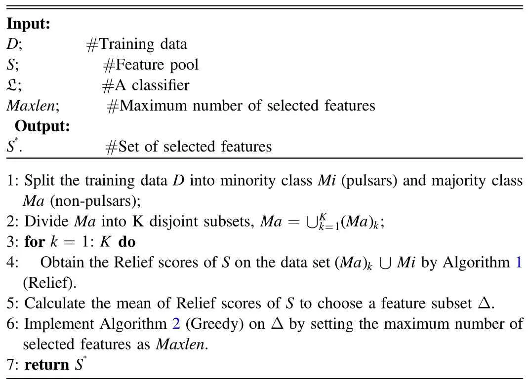
L Input:D; #Training data S; #Feature pool;#A classifier Maxlen; #Maximum number of selected features Output:S*.#Set of selected features 1: Split the training data D into minority class Mi (pulsars) and majority class Ma (non-pulsars);2: Divide Ma into K disjoint subsets, Ma Ma ;∪kK k= =3: fork=1:Kdo 4: Obtain the Relief scores of S on the data set Ma Mi 1( )( ) ∪ by Algorithm 1(Relief).5: Calculate the mean of Relief scores of S to choose a feature subset Δ.6: Implement Algorithm 2 (Greedy) on Δ by setting the maximum number of selected features as Maxlen.7: return S*k

5.Experiments and Analysis

In this section, experiments based on KFRG were implemented on HTRU.First, selected features by KFR and KFRG were calculated.Then, to demonstrate the improvement of KFRG,an ablation study was conducted to see the contribution of the component to the KFRG.Afterwards, comparative experiments with different feature groups were carried out to verify the effectiveness of KFRG.Finally, comparative experiments between our proposed KFRG and oversampling approaches were executed, and their advantages and disadvantages of each are discussed.

5.1.Results of KFG and KFRG

5.1.1.Selected Features Based on KFR Scores

The KFR algorithm is the first stage of Algorithm 3, which outputs the mean of Relief scores of the K-fold training sets.The Relief scores standing for the weights of features were calculated and are shown by a bar graph in Figure 3 for HTRU,where both the scores and their ranks are given.To select the more relevant features,a preset threshold will keep the features with higher scores.Here,a ratio of 0.618 is preset to ensure that the number of selected features is more than half of the total number of candidate features.That is, about 12 features out of 22 are considered to be very relevant(blue bars)and 10 others(gray bars) are less relevant.

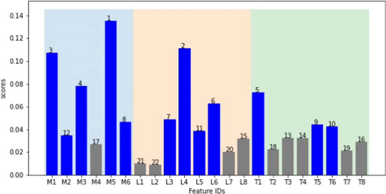
Figure 3.A bar graph of K-fold Relief scores of 22 features and their ranks on HTRU.A higher Relief score implies a more important feature.With a preset ratio,all features are divided into relevant ones (blue bars) and others (gray bars).

5.1.2.Selected Features Based on KFRG

Based on KFRG(Algorithm 3),the selected features as well as their size were obtained and the results are displayed in Table 3.

1.The dimension of features is greatly reduced.Most of the features in the feature pool were removed after applying the KFRG algorithm.The dimension of the selected features is cut down from 22 to less than eight.Some classifiers even need only three features to build their models.

2.The selected features and their sizes vary with the classifiers.For example, only three features, M5, L4 and T5, were finally chosen for DT while five features, M2,M3, M5, L4 and T1, were left for RF.

3.Features M5 and L4 are frequently used in all of the classifiers.It is shown that features M5 from Morello et al.(2014) and L4 from Lyon et al.(2016) are frequently selected.Further discussion is given in Section 6.

5.2.Ablation Study of KFRG

KFRG feature selection algorithm is an improvement of the Relief algorithm by combining KFR with a greedy algorithm.To demonstrate the effectiveness of KFRG, an ablation study of stack mode is given.Step by step, the performance metrics of all the classifiers were calculated from Relief to KFR, and finally, to KFRG.

Table 3 Selected Features Based on the KFRG Algorithm

Table 4 gives the numerical calculation of recall, precision,F1score and FPR for each classifier with three different feature select algorithms—-Relief, KFR and KFRG, while Figure 4 plots their averaged performance metrics.It shows that KFR performs better than Relief,and KFRG performs best of all.For one thing, KFR has better recall rates, better precision and lower FPRs for all classifiers than the original Relief techniques.For example, the recall raises from 94.8% to 96.1%.These improvements come from the step of K-fold Relief operation, as KFR is designed for the imbalance problem.For another aspect, KFRG keeps a precision rate as high as KFR,and raises the recall rate by 0.9%.Further,KFRG achieves a best F1score of 97.5%.These improvements come from the step of Greedy as it aims to maximize the F1score by removing the redundant features.

5.3.Comparison of Performance with Different Features

To verify the effectiveness of KFRG, comparative experiments with different feature groups were carried out, where three subsets of the feature pool were considered as the inputs of the classifiers,including features from Morello et al.(2014),features from Lyon et al.(2016)and features from KFRG.The performance metrics of recall (Rec), precision (Pre), F1score and FPR are expressed in Table 5.

Figure 4.The average performance metrics of Relief, KFR and KFRG.

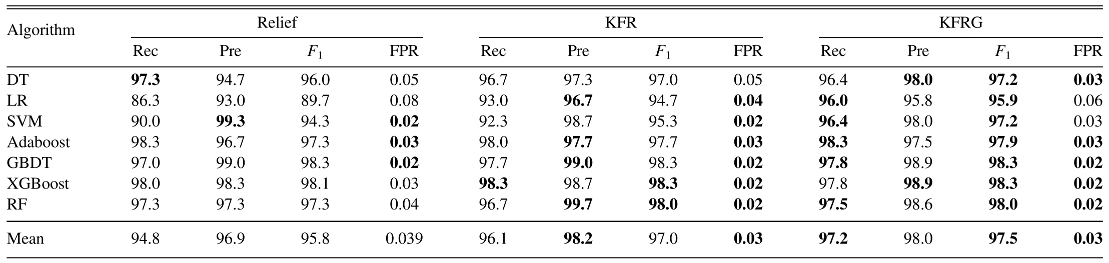
Table 4 Ablation Study of KFRG

The experimental results in Table 5 are summarized as follows.

1.Both the recall and precision have significantly improved.

The average recall of the classifiers is 97.2%, and most of the classifiers achieve recall rates ranging from 96% to 99% after applying the KFRG algorithm, which implies that most of the real pulsar signals were well detected after feature selection.For instance, the recall rate and the precision rate of DT are respectively 89.7%and 95.4% with features M1–M6, while they are up to 96.4% and 98% based on KFRG.Also, the average precision is as large as 98.0%based on KFRG,which has increased by an average of 3.9%compared with M1–M6 and L1–L8.

2.The FPR of the classifiers is reduced to 0.05% on average.

Most of the classifiers achieve an FPR less than 0.05%.A low FPR of a classifier implies that the selected features are very sensitive in excluding non-pulsars.

3.F1 scores based on selected features have increased.

The best F1is 98.3% in our experiment in the following cases: using five selected features [M3, M5,L3, L4, T1], GBDT achieved a recall of 97.8% and a precision of 98.9%; Using another five selected features[M5,M6,L4,T1,T5],XGBoost also achieved a high F1score of 98.3%,which is as good as the GBDT classifier.A better F1score implies that both recall and precision increase since F1score is the harmonic mean of recall and precision.In other words, more potential pulsar signals are correctly recognized and fewer non-pulsar signals are misjudged in these cases.

Table 5 Performance Metrics Based on Different Features,Including M1–M6 from Morello et al.,L1–L8 from Lyon et al.and the Selected Features by our Proposed KFRG Algorithm (Table 3), Where Rec, Pre, F1 and FPR Stand for Performance Metrics of Recall, Precision, F1 Score and FPR

5.4.Comparison of Performance with Different Databalancing Techniques

As feature selection of KFRG alleviates the imbalance problem on ML, the performances based on KFGR were compared with some other widely used data-balancing techniques of oversampling, including random oversampling,SMOTE (Chawla et al.2002), Borderline SMOTE (Han et al.2005) and ADASYN (He et al.2008).Furthermore, we even implement the KFRG-SMOTE method which is a combination of the proposed KFRG and SMOTE techniques.We evaluated the metrics of each algorithm on the different classifiers, and then took the mean of the performance of each classifier on each evaluation statistic to compare between feature selection metrics and oversampling metrics (Table 6).

It shows that KFRG offers better performance than oversampling techniques such as SMOTE,Borderline SMOTE and ADASYN, and random oversampling performs worst among them.KFRG achieves a similar recall rate but an improved precision and a lower FPR, which imply that the classifiers on KFRG are very strict in the criteria for classifying the candidates as pulsars and only a few of the non-pulsars were misjudged.Moveover,the performance of KFRG-SMOTE is as good as KFGR, which shares a high F1score of 97.5% and whose FPRs both range at a low level between 0.03%and 0.04%.

Compared with oversampling techniques,KFRG has its own advantages.One of the advantages is that KFRG has good generalization ability and is able to avoid overfitting problems.In fact, random oversampling tends to suffer from overfitting problems as the minority of samples in its training set were duplicated at random.As a result, the trained model becomes too specific to the training data and may not generalize well to new data.Other oversampling techniques are all based on SMOTE, which eliminates the harms of a skewed distribution by creating new minority class samples.They generate a synthetic sample xnewby using the linear interpolation of x and y with the expression of xnew=x+(y-x)×α, where α is a random number in the range[0,1]and y is a k-nearest neighborof x in the minority set.However, in many cases the kNNbased approach may generate wrong minority class samples as the above equation says that xnewwill lie in the line segment between x and y.In addition, it would be difficult to find an appropriate value of k for kNN a priori.The parameter k varies with the distribution of samples between minority and majority.Different from data-level methods of oversampling, feature selection of KFGR neither duplicates nor generates any additional data.It keeps the distribution and class IR of the data.

Table 6 Performance Metrics with Different Data-balancing Techniques, Including Random Oversampling, SMOTE, Borderline SMOTE, ADASYN, our Proposed KFRG Algorithm and KFRG-SMOTE Which is a Combination of the Proposed KFRG with SMOTE

The other advantage is that the result of KFRG is interpretable.The selected features are the most distinguishing ones between pulsars and non-pulsars.In addition, KFRG performs well based on the data characteristics regardless of the classifier used.Although the sets of selected features by KFRG may be changed with different classifiers, most of the selected features are the same, as will be explained in the next section.

6.Discussion

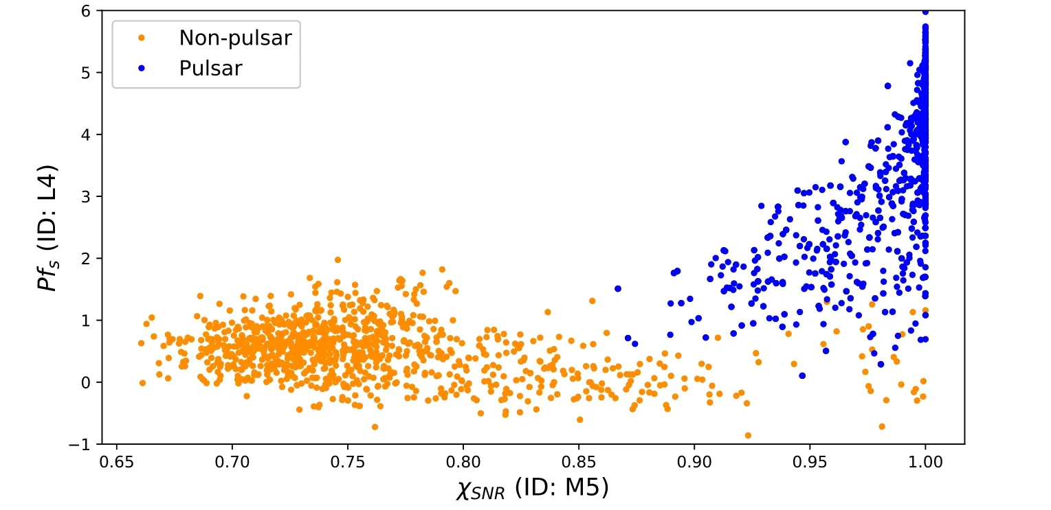
Figure 5.A scatter plot with coordinates of Feature M5 and L4.

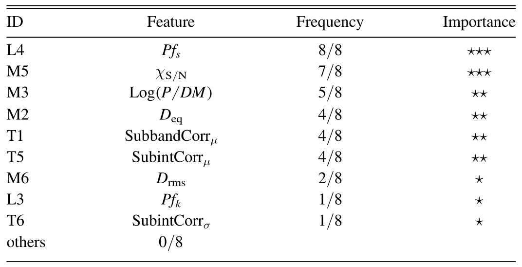
Table 7 Importance of the Selected Features

KFRG has been evaluated on HTRU.It demonstrates that models based on KFRG achieve larger recall, precision, F1score and less FPR than those without any feature selection.In other words,these selected features are distinguishable enough to pick out pulsar signals from the candidates.The improvement of performance metrics comes from two reasons.For one thing, the Relief algorithm can filter out most of the irrelevant features from the feature pool.As we have explained, Relief score is based on the identification of feature value differences between nearest neighbor instance pairs with both the same class and different classes.Thus, a feature with lower Relief score implies that the overlapping part of the two categories is large on the feature, which is considered as an irrelevant feature.Moreover,KFRG enables a classifier to select its most relevant features in a greedy way,as its objective function is to maximize the F1score of a given classifier.

Although the features selected by KFRG may be various for different classifiers, the most relevant features are almost the same.The importance of features was evaluated by their frequency of being selected and ranked with stars according to the KFRG results(Table 7).Features M5 and L4 are three star,as they are definitely selected by all the classifiers.Features M3,M2,T1 and T5 are ranked as two star, as they are chosen by about half of these classifiers.Features selected by only one or two classifiers are marked with one star.Those features left were never chosen by KFRG, implying they are redundant or irrelevant according to our experiments.

Notice that L4 and M5 are the most important features for most of the classifiers.They will be discussed in detail.L4 is the other feature that is the most relevant for all the classifiers.It notes the skewness on the folded profile (Pfs), which is a statistical value for the distribution of the pulse folded profile

where μ and σ are the mean and standard deviation of pi,respectively.A candidate with large L4 implies that there is a great skewness in the folded profile.Skewness describes the symmetry of the distribution of a signal.A signal with a great skewness is likely a signal with a distinctly detectable pulse.

M5, standing for χ(S/N), represents the persistence of the signal in the time domain,which is defined as the average score of χ(s)(Morello et al.2014), i.e.,, and

where s is the S/N of the candidate in a sub-integration, andpresents the benchmark of the S/N,where nsubis the total number of sub-integrations.The design basis of M5 is the fact that a genuine pulsar is expected to be consistently visible during most of an observation.As for artificial signals like RFIs,most of them last for a very short time,and then become invisible in a part of the observation.Therefore, M5 provides an effective selection criterion against these impulsive artificial signals.

A scatter plot with coordinates of Feature M5 and L4 in Figure 5 shows that: most of the non-pulsars can be easily separated from pulsars with these two features, as candidates with large L4 and M5 tend to be judged as pulsars.That could explain why they are frequently selected by most of the classifiers and are very significant for the PCS.

In this work, a novel feature selection algorithm KFRG is proposed to improve the performance of PCS models in the class-imbalanced case.KFRG combines Relief scores with the Greedy algorithm to remove most of the redundant and irrelevant features.Experiments based on HTRU show that KFRG is effective.Compared with models without any feature selection,the recall rate of the models based on KFRG features is higher and the FPR is lower.Compared with some typical oversampling techniques, KFRG is more robust and interpretable besides having better performance metrics.Also, the importance of selected features by KFRG is described and explained in our work.

These experimental conclusions based on KFRG are efficient and practical,providing a potential guide to study ML methods for candidate sifting, and serving other surveys of nextgeneration radio telescopes.

Acknowledgments

Authors are grateful for support from the National Natural Science Foundation of China(NSFC,grant Nos.11973022 and 12373108), the Natural Science Foundation of Guangdong Province (No.2020A1515010710), and Hanshan Normal University Startup Foundation for Doctor Scientific Research(No.QD202129).

Data Availability

The data underlying this article are publicly available in Centre for Astrophysics and Supercomputing, at http://astronomy.swin.edu.au/～vmorello/, which was released by Morello et al.(2014).The detailed description of the data is in Section 2.1.

ORCID iDs

Haitao Lin https://orcid.org/0000-0002-1441-9422