CAS FGOALS-f3-H Dataset for the High-Resolution Model Intercomparison Project (HighResMIP) Tier 2

Bo AN, Yongqiang YU*, Qing BAO, Bian HE, Jinxiao LI, Yihua LUAN,Kangjun CHEN, and Weipeng ZHENG

1State Key Laboratory of Numerical Modeling for Atmospheric Sciences and Geophysical Fluid Dynamics,Institute of Atmospheric Physics, Chinese Academy of Sciences, Beijing 100029, China

2College of Earth and Planetary Sciences, University of Chinese Academy of Sciences, Beijing 100049, China

ABSTRACT Following the High-Resolution Model Intercomparison Project (HighResMIP) Tier 2 protocol under the Coupled Model Intercomparison Project Phase 6 (CMIP6), three numerical experiments are conducted with the Chinese Academy of Sciences Flexible Global Ocean-Atmosphere-Land System Model, version f3-H (CAS FGOALS-f3-H), and a 101-year(1950-2050) global high-resolution simulation dataset is presented in this study. The basic configuration of the FGOALSf3-H model and numerical experiments design are briefly described, and then the historical simulation is validated. Forced by observed radiative agents from 1950 to 2014, the coupled model essentially reproduces the observed long-term trends of temperature, precipitation, and sea ice extent, as well as the large-scale pattern of temperature and precipitation. With an approximate 0.25° horizontal resolution in the atmosphere and 0.1° in the ocean, the coupled models also simulate energetic western boundary currents and the Antarctic Circulation Current (ACC), reasonable characteristics of extreme precipitation,and realistic frontal scale air-sea interaction. The dataset and supporting detailed information have been published in the Earth System Grid Federation (ESGF, https://esgf-node.llnl.gov/projects/cmip6/).

Key words:HighResMIP, FGOALS-f3-H, coupled model, data description, CMIP6

1.Introduction

Refinement of model resolution to enhance the fidelity of model simulation is one of the major evolving directions to further develop and optimize global coupled climate models, aiming to improve short-term climate prediction and climate change projections (Hewitt et al., 2017). For long-term simulations in climate studies, limited by the current state of computing resources, global coupled climate models with resolutions of at least 50 km in the atmosphere and 25 km in the ocean are referred to as relatively high-resolution models(Haarsma et al., 2016). The baroclinically unstable oceans of the world are rich with mesoscale eddies having radius scales smaller than 100 km (Chelton et al., 2011), exerting their impacts on the ocean and the atmosphere above (Small et al., 2008). These processes are parameterized or muted in typical CMIP5/CMIP6 coarse-resolution climate models(about 100 km resolution in the atmosphere and ocean), representing one of the main causes of uncertainty in climate projection. The high-resolution climate models can resolve mesoscale eddies in most of the ocean (apart from shallow bathymetry and polar regions) and better simulate the synoptic processes in the atmosphere (Delworth et al., 2012; Hallberg, 2013), provide a better representation of key processes(Griffies et al., 2015), and potentially offer more robust projections and predictions of climate variability and change(Haarsma et al., 2016; Hewitt et al., 2017). High-resolution models show significant improvements in simulating the mean state in the atmosphere and ocean, more realistic small-scale phenomena, and a better representation of extreme events such as heatwaves and floods. Increases in high-performance computing (HPC) resources enable the development of high-resolution global climate models in a growing number of climate research centers. Due to the expensive computational cost required by running high-resolution climate models, they are usually integrated only for multi-decadal to centennial model timescales, as oppossed to several thousand model years as is common with coarseresolution models.

The High-Resolution Model Intercomparison Project(HighResMIP) (Haarsma et al., 2016) is an endorsed project of Coupled Model Intercomparison Project 6 (CMIP6) by the World Climate Research Program (WCRP) (Eyring et al., 2016). For the first time, a coordinated effort in the highresolution CMIP modeling community aims to systematically investigate the impact of horizontal resolution by a multimodel approach. The standard for high resolution in High-ResMIP is 25-50 km for the atmosphere model and 10-25 km for the ocean model. The main experiments of High-ResMIP are divided into Tiers 1, 2, and 3. Tier 1 and Tier 3 are atmosphere-only runs, with the force of prescribed sea surface temperature and sea ice concentration. Tier 2 is a series of coupled experiments, which is more challenging in skills and computing resources. The period of coupled simulations is 1950-2050, which contains a 101-year control simulation(control-1950), a historical simulation from 1950 to 2014(hist-1950), and an RCP8.5 projection from 2015 to 2050(highres-future). For the HighResMIP Tier 2, there are currently 13, 11, and 9 simulations with high-resolution models for hist-1950, control-1950, and highres-future experiments uploaded to the ESG node, respectively.

The FGOALS (Flexible Global Ocean-Atmosphere-Land System Model) platform (Yu et al., 2002, 2004, 2011;Bao et al., 2010, 2013; Li et al., 2013) is a family of fully coupled climate system numerical models developed in the State Key Laboratory of Numerical Modeling for Atmospheric Science and Geophysical Fluid Dynamics, Institute of Atmospheric Physics, Chinese Academy of Sciences(LASG/IAP, CAS), and one of the latest versions f3-H(FGOALS-f3-H) contributes to the HighResMIP experiments. Over the past decades, the FGOALS family models have been widely applied in climate research and have actively contributed to climate modeling projects, including CMIP (Zhou et al., 2018). The third generation of FGOALS consists of three versions, e.g., FGOALS-g3, FGOALS-f3-L, and FGOALS-f3-H (He et al., 2019; Guo et al., 2020; Li et al., 2020a). Among these three versions, FGOALS-f3-H is configured with the highest resolution, namely about 0.25°resolution and 0.1° resolution in the atmosphere and ocean models, respectively. All Tier 1, 2, and 3 experiments of High-ResMIP with FGOALS-f3-H are conducted and submitted to the CMIP6 website, and the Tier 1 and 3 experiments are finished first (Bao et al., 2020), then the Tier 2 (coupled ocean-atmosphere simulations) experiment is finished afterward.

Here, we provide an overview of the FGOALS-f3-H simulation for the HighResMIP Tier 2 experiments. The remainder of this paper is structured as follows. Section 2 introduces the FGOALS-f3-H model description and the HighResMIP Tier 2 experimental design. Section 3 presents the validation of the dataset, and finally, section 4 shows data records and usage notes. Section 5 is summary.

2.Model experiments and observation data

2.1.Model description

FGOALS-f3-H is a fully coupled climate system model,which includes the atmospheric component model-version 2.2 of the Finite-volume Atmospheric Model of IAP/LASG(FAMIL2.2) (He et al., 2019; Bao et al., 2020; Li et al.,2021); an ocean component model-version 3 of the LASG/IAP Climate system Ocean Model (LICOM3.0) (Li et al., 2020b); a land component model-version 4.0 of the Community Land Model (CLM4.0) (Lawrence et al., 2011);and a sea-ice component model-version 4 of the Community Ice Code (CICE4.0) (Hunke and Lipscomb, 2010). The coupler is version 7 of the coupled module (Craig et al., 2012)from the National Center for Atmospheric Research(NCAR).

The atmospheric component, FAMIL2.2, is the latest version of the Finite-volume Atmospheric Model of the IAP/LASG (FAMIL) (Bao and Li, 2020; Li et al., 2021). A finite-volume dynamical core on a cubed sphere grid (Zhou et al., 2015) was employed in FAMIL2.2, with six tiles across the globe. In FAMIL2.2, each tile contains 384 grid cells (C384). Globally, the longitudes along the equator are divided into 1440 grid cells, and the latitudes are divided into 720 grid cells, which is approximately equal to a 0.25°horizontal resolution. The model uses a hybrid coordinate over 32 layers in the vertical direction, with the model top at 1 hPa. The physical schemes employed in FAMIL2.2 are documented (He et al., 2019; Bao et al., 2020). A scaleaware resolving convective precipitation parameterization(RCP) is used in FAMIL2.2 (Bao and Li, 2020).

The oceanic component, LICOM3.0, is the third version of the LASG/IAP Climate System Ocean Model (LICOM)(Zhang and Liang, 1989; Liu et al., 2012; Yu et al., 2018).An arbitrary orthogonal curvilinear coordinate dynamical core is introduced in the model (Yu et al., 2018) to apply the tripolar grid as suggested by Murray (1996). In LICOM3.0, the North Pole is relocated on the Eurasian (55°N, 95°E) and North American (55°N, 85°W) continents,respectively, which eliminates the singularity of the primitive equations in the North Pole and improves the simulation of the Arctic Ocean circulation (Li et al., 2017). Globally, the zonal circle is divided into 3600 grid cells, and the meridional circle from the North Pole to the Antarctic continent is divided into 2302 grid cells, which is approximately equal to a 0.1° horizontal resolution near the equator and smoothly increased to 0.05° or so in high latitudes. In the vertical direction, the model contains 55 levels with a nearly uniform depth of about 5 m in the top 10 layers. The physical package employed in LICOM3.0 is documented in Li et al.(2020b). Sub-grid parametrization schemes employed in LICOM3.0 include the tidal mixing scheme (St. Laurent et al., 2002; Yu et al., 2017), a buoyancy frequency related thickness diffusivity scheme (Ferreira et al., 2005), a vertical viscosity and diffusion scheme (Canuto et al., 2001), and a chlorophyll-a dependent solar penetration scheme (Lin et al.,2007), etc.

The land model CLM4 (Lawrence et al., 2011) has a 0.31° × 0.23° longitude-latitude grid resolution. The sea-ice model CICE4 (Hunke and Lipscomb, 2010) has the same grid system and land-sea mask as LICOM3.0. Several codes have been adjusted to adapt to the 3600 × 2302 tripolar grid.The sea ice in CICE4 is divided into five categories according to ice thickness in each grid cell to better simulate freezing and melting processes.

High-frequency coupling is required for high-resolution coupled runs: the coupled time step is 15 minutes between the coupler and the atmosphere, land, and sea ice model components, separately, and four hours between the coupler and the ocean model component.

2.2.Experimental design

The period of the HighResMIP (Haarsma et al., 2016)Tier 2 (coupled simulations) is 1950-2050, including three experiments: control-1950, hist-1950, and highres-future.Each experiment has only one ensemble member.

2.2.1.Control-1950

Here, control-1950 is the HighResMIP control experiment, which uses a fixed 1950s forcing. The forcing consists of GHG gases, including ozone and aerosol loading specific to the 1950s (～10-year mean) climatology.

The EN4 analyzed ocean state, representative of 1950,is used as the initial condition for temperature and salinity(Good et al., 2013). To reduce initial model drift, FGOALSf3-H first runs for 100 years with a constant 1950s forcing for spin-up, as recommended in the experimental design(Haarsma et al., 2016). Then, the model is run for another 101 years with the same forcing, the results of which are submitted to the CMIP6 website as the control-1950 simulations.

2.2.2.Hist-1950

Hist-1950 signifies the coupled historical runs for 1950-2014 using an initial condition taken from control-1950. For this period, the external forcings are the same as in HighResMIP Tier 1 (atmospheric-only runs).The anthropogenic aerosol forcing comes from the MACv2.0-SP model (Stevens et al., 2016), and the land use is fixed in time (Haarsma et al., 2016). Natural aerosol forcing, greenhouse gas concentrations, solar variability, and ozone forcing are the main standard forcing parameters for the CMIP6 historical simulations (Eyring et al., 2016).

2.2.3.Highres-future

Highres-future signifies the coupled scenario simulations, 2015-50, which are effectively a continuation of the hist-1950 historical simulation projected into the future.The forcing fields are based on the Representative Concentration Pathway 8.5 (RCP8.5) for the future period.

2.3.Observation, reanalysis, and other model data

Observation and reanalysis data are used to evaluate the model output. The 1950-2014 monthly sea-surface temperatures come from the Hadley Centre Sea Ice and Sea Surface Temperature dataset (HadISST), with a spatial resolution of 1° × 1°(Rayner et al., 2003) (https://www.metoffice.gov.uk/hadobs/hadisst/), and the IAP global ocean temperature gridded product at a 1° × 1° horizontal resolution (IAP_T)(Cheng et al., 2017) (http://www.ocean.iap.ac.cn/pages/dataService/dataService.html?navAnchor=dataService). The 1982-2014 monthly sea surface temperature (SST), with a spatial resolution of 0.25° × 0.25°, is from the NOAA 0.25°degree Daily Optimum Interpolation Sea Surface Temperature (OISSTv2.1) (Huang et al., 2021) (https://www.ncei.noaa.gov/products/optimum-interpolation-sst). The 1979-2014 monthly precipitation, with a spatial resolution of 2.5° ×2.5°, is from the Global Precipitation Climatology Project(GPCP) v2.3 (Adler et al., 2018) (http://gpcp.umd.edu/).The 1958-2014 monthly surface air temperature (at 2 m),with a spatial resolution of 1.25° × 1.25°, is from the Japanese 55-year Reanalysis (JRA-55) (Kobayashi et al.,2015) provided by the Japan Meteorological Agency (JMA),and the Central Research Institute of Electric Power Industry(CRIEPI). This dataset was also collected and provided under the Data Integration and Analysis System (DIAS),developed and operated by a project supported by the Ministry of Education, Culture, Sports, Science, and Technology(https://jra.kishou.go.jp/JRA-55/index_en.html#manual).The 1978-2014 monthly sea ice concentration, with a spatial resolution of 25 km × 25 km, is from NOAA/NSIDC Climate Data Record (CDR) of Passive Microwave Sea Ice Concentration, Version 4 (Windnagel et al., 2021) (https://nsidc.org/data/G02202/versions/4). The 1993-2014 monthly absolute dynamic topography of the Ssalto/Duacs altimeter products,with a spatial resolution of 0.25°, is from the Archiving, Validation, and Interpretation of Satellite Oceanographic data(AVISO). The Ssalto/Duacs altimeter products were produced and distributed by the Copernicus Marine and Environment Monitoring Service (CMEMS) (http://www.marine.copernicus.eu). (https://doi.org/10.48670/moi-00148). The 2000-20 3-h precipitation data, with a spatial resolution of 0.1°, is one of the satellite-retrieved products from Global Precipitation Measurement (GPM) (Huffman et al., 2014)(https://gpm.nasa.gov/data/directory).

CMIP6 historical simulation results from the lower resolution model FGOALS-f3-L (Guo et al., 2020) are used to compare with FGOALS-f3-H. Information concerning these models is given in Table 1.

Table 1. Model information of FGOALS-f3-H and FGOALS-f3-L.

3.Data validation of hist–1950 experiment

3.1.Temporal evolution of SST, precipitation, surface temperature, and sea ice extent

To illustrate the ability of FGOALS-f3-H to reproduce past climate change, we compare the simulated long-term time series of global mean with the observations and the lower resolution FGOALS-f3-L. The temporal evolutions of the globally averaged Sea Surface Temperature (SST) of FGOALS-f3-H are evaluated against HadISST and IAP_T(Fig. 1a). FGOALS-f3-H successfully captured the global mean SST increase over the historical period 1950-2014[0.059°C (10 yr)-1in FGOALS-f3-H, 0.065°C (10 yr)-1in HadISST and 0.09°C (10 yr)-1in IAP_T], with more rapid warming occurring in recent decades 1982-2014 [0.12°C(10 yr)-1in FGOALS-f3-H, 0.074°C (10 yr)-1in HadISST and 0.12°C (10 yr)-1in IAP_T]. Compared to FGOALS-f3-L, the globally averaged SST is about 0.6°C higher in FGOALS-f3-H. In FGOALS-f3-H, the SST increase is slower than in FGOALS-f3-L [0.10° C (10 yr)-1during 1950-2014 and 0.16°C (10 yr)-1during 1982-2014 in FGOALS-f3-L] and closer to the observed warming trend.

The temporal evolution of the globally averaged precipitation of FGOALS-f3-H and FGOALS-f3-L is evaluated against GPCPv2.3 (Fig. 1b). These two coupled models show higher precipitation by about 0.3 mm d-1and 0.16 mm d-1than observations, respectively, without any significant long-term trend.

The temporal evolutions of the global mean surface air temperature (at 2 m) of FGOALS-f3-H and FGOALS-f3-L are evaluated against JRA-55 (Fig. 1c). FGOALS-f3-H reproduces the increase in the global-scale annual mean surface temperature over the historical period 1950-2014 [0.1°C(10 yr)-1in FGOALS-f3-H, 0.12°C (10 yr)-1in JRA-55 during 1958-2014], including the more rapid warming during 1982-2014 [0.18°C (10 yr)-1in FGOAS-f3-H, 0.13°C(10 yr)-1in JRA-55]. It also reproduced the abrupt cooling immediately following large volcanic eruptions, like the 1991 Pinatubo eruption. The global averaged 2-m air temperature is about 0.7°C higher in FGOALS-f3-H than FGOALSf3-L. Compared to FGOALS-f3-L, the surface air temperature warming rate is slower in FGOALS-f3-H, closer to JRA-55[0.17°C (10 yr)-1during 1950-2014 and 0.24°C (10 yr)-1during 1982-2014 in FGOALS-f3-L].

Fig. 1. Timeseries of annual global mean (a) SST (units: °C) (b) precipitation (units: mm d-1)(c) 2-m air temperature (units: °C) from FOGALS-f3-H (black), FGOALS-f3-L (green) and observation or reanalysis data (red and blue) during 1950-2014. Timeseries of (d) Arctic sea ice extent (units: 106 km2) and (e) Antarctic sea ice extent (units: 106 km2) in March (solid)and September (dashed), from FOGALS-f3-H (black), FGOALS-f3-L (green) and observation data (Bootstrap in red and Passive Microwave in blue) during 1950-2014.

The sea ice extent (area covered by ice with a concentration above 15%) in March and September from FGOALSf3-H and FGOALS-f3-L (Figs. 1d-e) are evaluated against observations. FGOALS-f3-H shows an improved sea ice extent simulation in both the Arctic and Antarctic compared to FGOALS-f3-L. In the Arctic (Fig. 1d), FGOALS-f3-L overestimates the boreal winter (March) sea ice extent,FGOALS-f3-H well simulates both the boreal winter sea ice extent (about 11.6 ×106km2in FGOALS-f3-H and 12.6 ×106km2in observation) and the boreal summer (September)sea ice extent (about 4.5 × 106km2in FGOALS-f3-H and 5 ×106km2in observation). FGOALS-f3-H captures the decrease in sea ice extent over the past few decades(1979-2014) in the Arctic [-0.05 × 106km2(10 yr)-1and-0.18 × 106km2(10 yr)-1in FGOALS-f3-H, -0.4 (-0.03) ×106km2(10 yr)-1and -0.8 (-0.5) × 106km2(10 yr)-1as indicated by passive microwave (bootstrap), for boreal winter and summer, respectively]. In the Antarctic (Fig. 1e),FGOALS-f3-L underestimates the austral summer (March)sea ice extent, FGOALS-f3-H well simulates the austral summer sea ice extent (about 2 × 106km2in FGOALS-f3-H and 3 × 106km2in observation). Still, it underestimates the austral winter (September) sea ice extent (about 11.6 × 106km2in FGOALS-f3-H and 16 × 106km2in observation). The simulated Antarctic sea ice extent shows a slight decreasing trend.

3.2.Mean state bias of SST, precipitation, and surface temperature

The climatological annual mean SST of FGOALS-f3-H is compared with OISSTv2.1 (Fig. 2a). FGOALS-f3-H reproduces observed large-scale mean sea surface temperature patterns with a bias of less than 1.5°C in most regions. Locations with large biases include a cold bias in South Atlantic and warm biases in the North Atlantic and Antarctic Circumpolar Current (ACC), consistent with the underestimated sea ice extent in both hemispheres, as shown in Figs. 1d-e. The cold SST biases in midlatitude North Pacific are smaller in FGOALS-f3-H compared to FGOALS-f3-L, while the warm biases in the ACC seem larger (Fig. 2b). In the North Atlantic, there is a warm bias in FGOALS-f3-H, while a cold bias is present in FGOALS-f3-L.

Figure 2c shows the climatological annual mean precipitation rate from two coupled models against GPCPv2.3.FGOALS-f3-H well captured the large-scale features, such as the maximum precipitation centers to the north of the equator, in the central and eastern tropical Pacific, in the eastern tropical Atlantic, and the Indian Ocean. It also successfully simulated the dry areas over the eastern subtropical ocean basins and Northern Africa. At regional scales, the biases include greater precipitation in the maximum rain belt, excessive precipitation in tropical convergence zones south of the equator in the eastern Pacific, and lower precipitation in South America. FGOALS-f3-H shares a similar precipitation bias pattern with FOGALS-f3-L (Fig. 2d), with a larger magnitude. Bao et al. (2020) indicated that the high-resolution AMIP run already has a larger precipitation bias than the low-resolution one, which may result from a lack of specific tuning of the sub-grid parameterization schemes for the high-resolution AGCM. In this study, the initial precipitation bias in the stand-alone AGCM is further amplified in the coupled model due to air-sea interactions.

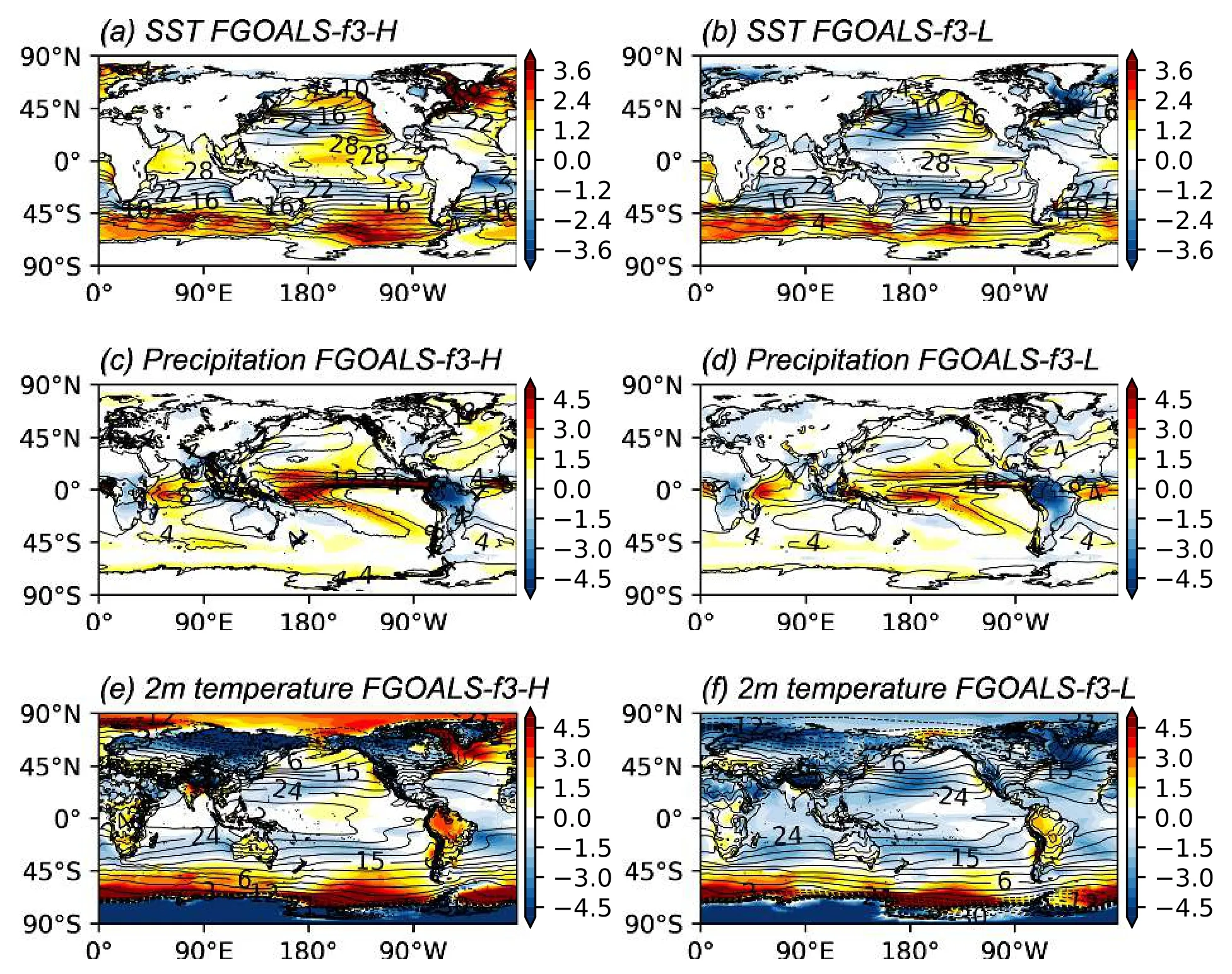
Fig. 2. (a) Climatological mean (lines) SST (units: °C) from FGOALS-f3-H and its bias (color) against OISSTv2.1 during 1982-2014, (c) climatological mean (lines) precipitation (units: mm d-1) from FGOALS-f3-H and its bias (color) against GPCP during 1979-2014, (e) climatological mean (lines) 2-m air temperature (units: °C) from FGOALS-f3-H and its bias(color) against JRA-55 during 1979-2014, (b), (d), (f) are the same but for FGOALS-f3-L.

The simulated climatological annual mean surface air temperature (at 2 m) is evaluated against JRA-55 (Fig. 2e).FGOALS-f3-H reproduces observed large-scale mean surface temperature patterns. In most areas, FOGALS-f3-H agrees with the reanalysis within 2°C. S till, there are several locations where the biases are much larger, particularly cold biases at high elevations over the Tibetan Plateau, Rocky Mountains, Antarctica, parts of both Greenland and Northern Asia, with warm biases in South Africa, near the Barents Sea, North Atlantic, and above the ACC. The pattern of bias over the ocean is consistent with the SST bias pattern.FGOALS-f3-H and FOGALS-f3-L show different 2-m air temperature bias patterns, with mostly cold biases in FGOALS-f3-L.

Fig. 3. Standard deviation of monthly SSH (units: cm) from (a) FGOALS-f3-L, (c) FOGALS-f3-H, and (e) AVISO during 1993-2014. Climatological monthly mean EKE (units: cm2 s-2) from (b) FGOALS-f3-L and (d) FGOALS-f3-H during 1993-2014.

3.3.Meso-scale Eddies

FGOALS-f3-H employs the eddy-rich ocean component model LICOM3.0, with 0.1° horizontal resolution, resolving the first Rossby radius of deformation over most of the ocean (Hallberg, 2013) and generating mesoscale eddies through barotropic and baroclinic instabilities. Therefore,FGOALS-f3-H enables a more nonlinear solution and, thus,a better representation of western boundary currents like Gulf Stream and Kuroshio. To show the amplitude of the mesoscale eddies, the standard deviation (STD) of sea surface height (SSH) of FGOALS-f3-H is evaluated against FGOALS-f3-L and AVISO (Figs. 3a, c, e). With increased resolution, there is a significant increase in the SSH variability that is close to the observations, which is also shown in the LICOM3.0 ocean-only runs (Li et al., 2020b). For the LICOM3.0 ocean-only runs, the high viscosity and damping effect are believed to result in underestimating SSH variability and eddy kinetic energy (EKE) compared to observations(Li et al., 2020b). Since frontal air-sea interactions are overestimated in the high-resolution ocean-only runs but are more realistic in coupled runs, the FGOALS-f3-H SSH variability is higher than the ocean-only runs, with western boundary current locations similar to observations. In FGOALS-f3-H,with the fully coupled high-resolution model, the variability is stronger than observations in the western boundaries and ACC in the Southern Hemisphere but lower in the ocean interiors. Figures 3b and 3d show the monthly mean surface EKE of FGOALS-f3-H and FGOLAS-f3-L. Significant increases in EKE are seen in the Kuroshio and Gulf Stream currents, the South Atlantic, the Agulhas Return Current,and the ACC in FGOALS-f3-H, indicating a much more energetic surface ocean.

3.4.Extreme Precipitation

Extreme precipitation remains a grand challenge in climate modeling, especially for extreme hourly precipitation.Figure 4 shows the 3-hourly precipitation intensity-frequency distribution in the model results of FGOALS-f3-H and GPM. Dai (2006) pointed out that these simulations usually tend to overestimate light rainfall (＜ 10 mm d-1) but underestimate heavy rainfall (＞ 20 mm d-1). FGOALS-f3-H easily overcomes such common biases, as illustrated in Fig. 4. The distribution of the light rainfall in the FGOALS-f3-H is wellmatched to GPM satellite products. As for the extreme precipitation [＞20 mm (3 h)-1], the distribution of intensity-frequency from FGOALS-f3-H is also quite consistent with GPM satellite products; however, events with precipitation over 80 mm (3 h)-1are underestimated to some extent. With high resolution and suitable physical processes in FGOALSf3-H, the simulated extreme precipitation intensity and distribution seem distinctly improved (He et al., 2019).

Fig. 4. The 3-hourly precipitation intensity-frequency distribution (units: %) in the model results of FGOALS-f3-H(blue) and the satellite retrieved products from Global Precipitation Measurement (GPM) (black).

3.5.Mesoscale air-sea interaction

The positive correlation between frontal and mesoscale near-surface wind speed and SST was first found from highresolution satellite observations (Xie, 2004; Small et al.,2008), which was surprising because, for larger basin scales,the correlation is often negative in extratropical regions. A negative correlation between near-surface wind speed and SST (meaning large wind speeds correspond with cold SSTs) would indicate that the atmosphere is driving an ocean response. Conversely, a positive correlation between near-surface wind speed and SST (meaning warm SSTs correspond with large wind speeds) would indicate that the ocean is driving an atmosphere response. Even for Bjerknes feedback which includes both atmosphere-forced oceanic processes and ocean-forced atmospheric processes, the correlation between near-surface wind speed and SST is negative.Bryan et al. (2010) then used this metric (positive correlation between SST and surface wind speed in the frontal and mesoscale) to test the fidelity of climate models with different resolutions and found that only the eddy-resolving models captured this characteristic of frontal scale ocean-atmosphere interaction. A more realistic pattern of positive correlation between small-scale features in SST and low-level wind speed is captured in FGOALS-f3-H (Fig. 5a), compared to the almost no correlation in FGOALS-f3-L (Fig. 5b). Figure 5 displays the global map of the temporal correlation between monthly spatial high-pass (spatial 3° × 3° boxcar filter) filtered surface wind speed (at 10 m) and SST of FGOALS-f3-H and FGOALS-f3-L. The filter is applied by first calculating the spatial 3° × 3° box average, then by using the difference between the original and averaged fields to get the high-pass fields to get the high-pass fields.FGOALS-f3-H shows significant positive correlations over regions with strong fronts and mesoscale eddies: the Gulf Stream, the Kuroshio and their extensions, and the ACC in the Southern Hemisphere. The correlation pattern in FGOALS-f3-H is very similar to observations in Bryan et al.(2010) and Lin et al. (2019). With an eddy-rich ocean component, the tropical instability waves (TIWs) become better resolved. Thus, FGOALS-f3-H shows a strong and spatially extensive positive correlation in the eastern Tropical Pacific(not shown). A few regions of significant negative correlation also persist in tropical areas in FGOALS-f3-H.

4.Data records and usage notes

The datasets of the HighResMIP Tier 2 experiments have been uploaded onto the ESG node and can be found at(https://esgf-node.llnl.gov/projects/cmip6/). The simulation year of each experiment is listed in Table 3. Please cite as follows: (CAS FGOALS-f3-H model output prepared for CMIP6 HighResMIP hist-1950. Earth System Grid Federation. https://doi.org/10.22033/ESGF/CMIP6.3316. CAS FGOALS-f3-H model output prepared for CMIP6 High-ResMIP control-1950. Earth System Grid Federation.https://doi.org/10.22033/ESGF/CMIP6.3216. CAS FGOALS-f3-H model output prepared for CMIP6 High-ResMIP highres-future. Earth System Grid Federation.https://doi.org/10.22033/ESGF/CMIP6.3302). The linear trends of the annual mean 2-m air temperature and annual mean precipitation from 2015 to 2050 in FGOALS-f3-H highres-future simulation are given in Fig. S1 in the electronic supplementary material (ESM).

Fig. 5. Temporal correlation of high-pass filtered surface wind speed with SST from (a)FOGALS-f3-H and (b) FGOALS-f3-L during 2001-08. Stippling indicates statistical significance at the 95% level calculated using a two-tailed Student t-test.

The model data are post-processed by CMOR software and saved in a single-precision Network Common Data Form version4 (NetCDF4), which can be processed by common computer programming languages and professional software, such as the Climate Data Operator (CDO, https://code.mpimet.mpg.de/projects/cdo/) and the NetCDF Operator.There are monthly mean outputs and daily mean outputs available in the datasets, especially high-frequency three-hourly mean and six-hourly transient outputs of atmospheric variables. The storage of variables follows the ESG protocol.The full list of all the output variables can be found by visiting the data repository on the ESG node (https://esgf-node. llnl.gov/projects/cmip6/). Table 2 provides an explanation of the priority variables. The full list of available variables,including the further variable information and downloading script, can be searched through the CMIP6 Search Interface(https://esgf-node.llnl.gov/search/cmip6/).

Table 2. Descriptions of dataset priority variables for HighResMIP. 3 h: 3 hourly mean samples; 6-hPlevPt: sampled 6 hourly, at specified time point within the time period; day: daily mean samples; mon: monthly mean samples; A for the atmospheric variables; and O for the oceanic variables.

Table 3. Years of FGOALS-f3-H HighResMIP Tier 2 simulations.

The original atmospheric model grid is in the cube sphere grid system, which has six tiles and is irregular in the horizontal direction. The data uploaded to ESG are post-processed by merging and interpolating the tiles onto a normal 0.25° global latitude-longitude grid, using a one-order conservation interpolation as required by CMIP6. For calculating pressure at the model layers, please refer to He et al. (2019).The land model outputs uploaded to ESG are on the native latitude-longitude grid.

The data of the oceanic model and sea-ice model uploaded to ESG are on the original tripolar grid. Users can read and visualize the original data by software that supports the curvilinear coordinate, like the NCAR Command Language (NCL, http://www.ncl.ucar.edu) or Python (https://www.python.org), or interpolate the data onto a normal latitude-longitude grid using software like CDO or NCO before use. For interpolation, the scalar variables can be directly interpolated, but the vector variables need to be rotated according to the angles between the native grid and the latitude-longitude grid before interpolation. Please refer to Yu et al. (2018) for the dynamic framework in LICOM3.0. The attributes of the tripolar grid, like the grid cell area, ocean depth, unit water mass, etc., are also provided in the datasets.

5.Summary

This paper introduces the HighResMIP Tier 2 experimental design and basic model configuration of climate system model CAS FGOALS-f3-H, briefly validates the historical results by comparing them with observation and lower resolution FGOALS-f3-L CMIP6 historical simulation, and gives usage notes about the dataset. Results show thatFGOALS-f3-H better reproduces the observed long-term trends of global temperature, precipitation, and sea ice extent, as well as the large-scale pattern of temperature and precipitation, simulates more energetic western boundaries and realistic meso-scale air-sea interaction. However, there are still some biases in the high-resolution simulation such as the over precipitation in the tropical region. The High-

ResMIP aims to evaluate the impact of horizontal resolution on model simulation and provides a variety of datasets with high-resolution climate models. In this respect, this paper provides some general information about the FGOALS-f3-H dataset for data users in the scientific community.

Acknowledgements. This study is jointly supported by the Strategic Priority Research Program of the Chinese Academy of Sciences (Grant Nos. XDA19060102 and XDB42000000) and National Natural Science Foundation of China (Grant Nos.91958201 and 42130608) and the National Key Research and Development Program of China (Grant No. 2020YFA0608800). This study was supported by the National Key Scientific and Technological Infrastructure project “Earth System Numerical Simulation Facility” (EarthLab).

Electronic supplementary material:Supplementary material is available in the online version of this article at https://doi.org/10.1007/s00376-022-2030-5.

Open AccessThis article is licensed under a Creative Commons Attribution 4.0 International License, which permits use, sharing,adaptation, distribution and reproduction in any medium or format,as long as you give appropriate credit to the original author(s) and the source, provide a link to the Creative Commons licence, and indicate if changes were made. The images or other third party material in this article are included in the article’s Creative Commons licence, unless indicated otherwise in a credit line to the material.If material is not included in the article’s Creative Commons licence and your intended use is not permitted by statutory regulation or exceeds the permitted use, you will need to obtain permission directly from the copyright holder. To view a copy of this licence,visit http://creativecommons.org/licenses/by/4.0/.