
Stochastically Perturbed Parameterizations for the Process-Level Representation of Model Uncertainties in the CMA Global Ensemble Prediction System
2022-11-07 05:33:10FeiPENGXiaoliLIandJingCHEN
Fei PENG, Xiaoli LI*, and Jing CHEN
1 CMA Earth System Modeling and Prediction Centre, China Meteorological Administration (CMA), Beijing 100081
2 State Key Laboratory of Severe Weather, China Meteorological Administration, Beijing 100081
3 National Meteorological Centre, China Meteorological Administration, Beijing 100081
ABSTRACT To represent model uncertainties at the physical process level in the China Meteorological Administration global ensemble prediction system (CMA-GEPS), a stochastically perturbed parameterization (SPP) scheme is developed by perturbing 16 parameters or variables selected from three physical parameterization schemes for the planetary boundary layer, cumulus convection, and cloud microphysics. Each chosen quantity is perturbed independently with temporally and spatially correlated perturbations sampled from log-normal distributions. Impacts of the SPP scheme on CMA-GEPS are investigated comprehensively by using the stochastically perturbed parametrization tendencies(SPPT) scheme as a benchmark. In the absence of initial-condition perturbations, perturbation structures introduced by the two schemes are investigated by analyzing the ensemble spread of three forecast variables’ physical tendencies and perturbation energy in ensembles generated by the separate use of SPP and SPPT. It is revealed that both schemes yield different perturbation structures and can simulate different sources of model uncertainty. When initialcondition perturbations are activated, the influences of the two schemes on the performance of CMA-GEPS are assessed by calculating verification scores for both upper-air and surface variables. The improvements in ensemble reliability and probabilistic skill introduced by SPP and SPPT are mainly located in the tropics. Besides, the vast majority of the reliability improvements (including increases in ensemble spread and reductions in outliers) are statistically significant, and a smaller proportion of the improvements in probabilistic skill (i.e., decreases in continuously ranked probability score) reach statistical significance. Compared with SPPT, SPP generally has more beneficial impacts on 200-hPa and 2-m temperature, along with 925-hPa and 2-m specific humidity, during the whole 15-day forecast range. For other examined variables, such as 850-hPa zonal wind, 850-hPa temperature, and 700-hPa humidity, SPP tends to yield more reliable ensembles at lead times beyond day 7, and to display comparable probabilistic skills with SPPT. Both SPP and SPPT have small impacts in the extratropics, primarily due to the dominant role of the singular vectors-based initial perturbations.
Key words: model uncertainty, global ensemble forecast, stochastic physics, parameter perturbation, perturbation structure
1. Introduction
Ensemble prediction systems (EPSs) provide a useful tool to estimate the inherent uncertainties that exist in conventional single-model deterministic forecasts. It is well known that an EPS with initial-condition perturbations (IPs) alone tends to be underdispersive, thus yielding unreliable and overconfident ensemble forecasts(e.g., Buizza et al., 2005; Wilks, 2005; Zheng et al.,2019). Besides the initial conditions, another major source of forecast uncertainties is the model itself. Due to simplifications and approximations used in formulating numerical models, model uncertainties (i.e., model errors) inevitably exist. To further improve the reliability and probabilistic skills of EPSs, the role of model uncertainties has been drawing more and more attention. In recent years, stochastic physics schemes, which aim to represent model uncertainties that lie in the parameterizations of subgrid-scale physical processes, have been widely developed (Berner et al., 2017; Ollinaho et al.,2017; Christensen, 2020; Fleury et al., 2022). So far,these schemes have been put into use routinely to generate short-range, medium-range, and seasonal ensemble forecasts in many operational weather and climate centers, such as the ECMWF (Palmer et al., 2009), NCEP(Zhou et al., 2017), UK Met Office (Sanchez et al.,2016), and China Meteorological Administration (CMA;Chen and Li, 2020).
A range of stochastic physics schemes have been designed to represent the various sources of model uncertainties (Palmer et al., 2009; Berner et al., 2017; Fleury et al., 2022). According to the formulae of stochastic schemes, the representation of model uncertainties is usually achieved by incorporating a stochastically multiplicative or additive forcing term into the model. One of the most widely used schemes is the stochastically perturbed parameterization tendencies (SPPT) scheme, in which the net tendencies of physical parameterizations are multiplied by spatiotemporally correlated random perturbations (Buizza et al., 1999; Palmer et al., 2009).SPPT addresses uncertainties in parameterized physical tendencies related to sub-grid variability. For a global EPS, SPPT is known to be effective in improving both the ensemble reliability and the probabilistic skill, especially in the tropics (Palmer et al., 2009; Leutbecher et al., 2017; Li et al., 2019). In a limited-area EPS at mesoscale or convection-permitting scale, the scheme also has beneficial impacts through reducing errors and introducing additional ensemble spread (Bouttier et al., 2012;Romine et al., 2014; Yuan et al., 2016). In terms of additive forcing, a representative approach is the stochastic kinetic energy backscatter (SKEB) scheme (Shutts,2005), which was proposed to capture the upscale transport of energy associated with subgrid-scale processes otherwise missed in a truncated model. Through the addition of stochastic streamfunction and temperature forcing terms weighted by local energy dissipation rates into the model equations, this scheme can offset the energy loss arising from the truncated model equations, numerical diffusion, parameterized deep convection, and gravity drag. The positive role of SKEB has been reported in synoptic-scale, mesoscale, and convection-permitting ensembles (Berner et al., 2009; Tennant et al., 2011; Duda et al., 2016; Xu et al., 2020).
Unlike the SPPT and SKEB schemes, which provide bulk representations of model uncertainties, schemes that stochastically perturb uncertain parameters in the model physics have been developed to represent uncertainties at specified physical process levels (e.g., convection, turbulent diffusion), and are believed to be more directly linked to the model error sources (Leutbecher et al.,2017). In terms of the implementation of such schemes in related research, the selection of key parameters as well as the adopted perturbations can be dealt with in different ways based on the characteristics of the model used and the physical processes being investigated (Bowler et al., 2008; Hacker et al., 2011; Jankov et al., 2017, 2019;Leutbecher et al., 2017; Wang et al., 2019; Wastl et al.,2019). More specifically, during the model’s integration,the parameter perturbations can be kept unchanged in space and time, fixed in space but varied in time, or varied in both space and time, and these different variants are referred to as the multi-parameter scheme, the random parameter (RP) scheme, and the stochastically perturbed parameterization (SPP) scheme, respectively (e.g.,Bowler et al., 2008; Hacker et al., 2011; Leutbecher et al., 2017). The latter two (RP and SPP), as critical parts of stochastic physics schemes, have been widely applied in ensemble forecasts (e.g., Bowler et al., 2008; McCabe et al., 2016; Ollinaho et al., 2017). Owing to the incorporated perturbations without spatial variations, the RP scheme only considers the temporal uncertainty in parameters. Different from the RP scheme, the SPP scheme can simultaneously consider the temporal and spatial uncertainty by constructing temporally and spatially varying parameter perturbations. Ollinaho et al. (2017) introduced the SPP scheme in the ECMWF ensemble system by stochastically and independently perturbing 20 parameters and variables from the ECMWF Integrated Forecast System model physics package associated with turbulent diffusion, subgrid orography, convection, clouds,large-scale precipitation, and radiation. The applied perturbation patterns were characterized by variations and correlations in both time and space, and drawn from the normal or log-normal distributions. Their results revealed that SPP can generate more improvements when benchmarked against IPs only. However, when compared with SPPT, SPP showed comparable forecast skill at short-range lead times and lower skill at mediumrange lead times for upper-air variables. Similarly,Jankov et al. (2017) also applied SPP in a mesoscale ensemble system, built on the basis of the Weather Research and Forecasting model, by perturbing four key uncertain parameters in the convective and boundary schemes, and the additive impacts of combining SPP with other stochastic physics schemes such as SPPT and SKEB were generally positive.
The CMA global ensemble prediction system (CMAGEPS; initially known as GRAPES-GEPS; Chen and Li,2020; Shen et al., 2020) has been operationally running since December 2018. The SPPT and SKEB schemes have been implemented in CMA-GEPS to represent model uncertainties (Li et al., 2019; Peng et al., 2019),and both have been tuned to be effective in improving the ensemble performance. In addition, the implementation of SPPT is similar to that in the ECMWF ensemble system (Palmer et al., 2009), i.e., through multiplying the net physical tendencies for zonal wind, meridional wind,temperature, and humidity by a two-dimensional (2D)stochastic field correlated in space and time, and the addition of a tapering function dependent on the model level to retain numerical stabilities in the planetary boundary layer (PBL) and the relative accuracy of radiative tendencies in the stratosphere. Nonetheless, as demonstrated in many previous studies (Leutbecher et al., 2017; Lock et al., 2019; Christensen, 2020), SPPT has some drawbacks. For example, the conservation laws for energy and moisture are broken due to the mismatch between the perturbed tendencies and the unperturbed surface fluxes, as well as fluxes at the top of the atmosphere. The assumptions underlying SPPT are physically unreasonable to some extent, as the same random field in the vertical direction is used for the physical tendencies of all model variables (Christensen, 2020). Moreover, according to the assumptions of SPPT, large (small) uncertainties exist in larger (smaller) net physical tendencies,which is not always the truth (Leutbecher et al., 2017).These shortcomings also constitute one of the main reasons for efforts in the research and development of SPP at ECMWF, the purpose of which is to replace SPPT with SPP in the future (Leutbecher et al., 2017; Ollinaho et al.,2017; Lang et al., 2021).
Compared with SPPT, the SPP scheme has advantages in terms of respecting the conservation laws related to energy and moisture, as well as the physically consistent relationships between different model variables, and is thus deemed a more physically justified method (Leutbecher et al., 2017). To directly tackle model errors at their source and improve the ensemble performance through a more physically consistent representation of model uncertainties, in this study, the SPP scheme is introduced into CMA-GEPS by perturbing 16 key parameters in the physical parameterizations for the PBL, cumulus convection, and cloud microphysics, with stochastic fields exhibiting temporal and spatial correlation characteristics. Furthermore, the currently operational SPPT scheme in CMA-GEPS is used as a baseline to compare the perturbation features introduced by SPP and SPPT so as to clarify the differences between the two methods. In addition, the impacts of the two schemes on the forecast skill are analyzed and compared to illustrate the potential value of SPP for CMA-GEPS.
The structure of the paper is as follows. A brief introduction to CMA-GEPS, along with the detail of the SPP scheme and the design of the numerical experiment are presented in Section 2. Section 3 describes the perturbation structures introduced by SPP and SPPT in terms of model physical tendencies and perturbation energy. In Section 4, different verification scores are employed to evaluate and compare the impacts of SPP and SPPT on CMA-GEPS. Finally, Sections 5 and 6 provide some further discussion points and our conclusions, respectively.
2. Model, methods, and experimental design
2.1 CMA-GEPS
CMA-GEPS is a key part of the operational numerical weather prediction system developed by the CMA (Shen et al., 2020). It is built on the CMA global forecast system (CMA-GFS; initially known as GRAPES-GFS; Xue and Chen, 2008; Shen et al., 2020), which includes a non-hydrostatic dynamic core and an optimized suite of physical parameterizations for cumulus convection,cloud microphysics, vertical diffusion, radiation, and gravity drag. In addition, the physical package of CMAGFS consists of the new medium-range forecast (NMRF)PBL scheme (Hong and Pan, 1996; Chen et al., 2017,2020), the new simplified Arakawa–Schubert (NSAS)shallow and deep convection scheme (Arakawa and Schuber, 1974; Pan and Wu, 1995; Liu et al., 2015), a modified two-moment cloud scheme (Chen et al., 2007;Ma et al., 2018), and the RRTMG (Rrapid Radiative Transfer Model for General circulation models) longwave and shortwave radiation scheme (Pincus et al.,2003).
In CMA-GEPS, singular vectors (SVs) are used to account for uncertainties in the initial conditions (Li and Liu, 2019; Huo et al., 2020). Based on the tangent-linear approximation of the nonlinear forecast model at the horizontal resolution of 2.5° × 2.5°, the SVs are computed with the optimization time interval of 48 h in terms of the total energy norm, aimed at capturing the fastest linearly growing perturbations. IPs are constructed by linearly combining the SVs calculated for different target regions of the extratropical Southern Hemisphere (30°–80°S) and Northern Hemisphere (30°–80°N), as well as up to six tropical areas, centered on tropical cyclones in the Pacific, through a Gaussian sampling method. Currently, 15 combined SVs-based perturbations have been applied to generate 30 perturbed initial conditions by adding and subtracting these perturbations to the analysis fields. In this study, CMA-GEPS, with 31 members (including one control member), is run at the horizontal resolution of 0.5° × 0.5° with 60 vertical levels (model top at approximately 3 hPa) and a forecast length of 15 days. The SPPT and SKEB schemes are employed to mimic the uncertainties in the model itself (Li et al., 2019; Peng et al.,2019, 2020).
2.2 The SPP scheme in CMA-GEPS
The SPP scheme aims to account for model uncertainty at its source by directly perturbing a range of uncertain and vital parameters or variables from different model physics schemes. The choice of parameters or variables in this study is focused on three model parameterizations in CMA-GFS, for the PBL, cumulus convection, and cloud microphysics, based on related literature and suggestions from the CMA’s physics parameterization experts (Liu et al., 2015; Ollinaho et al., 2017; Chen et al., 2020). Table 1 illustrates the 16 selected parameters and variables to be perturbed, as well as their physical descriptions, default values, and possible variational ranges constrained by the minimum and maximum values. In CMA-GFS, the currently used PBL scheme is the NMRF PBL scheme, which is aK-closure, nonlocal vertical diffusion method (Hong and Pan, 1996; Chen et al.,2020). From this scheme, a total of six key parameters(P01–P06 in Table 1) related to the calculation of diffusivity coefficients, nonlocal counter-gradient terms, mixing length scales, and stratocumulus cloud simulations are perturbed to represent the uncertainty in modeling the PBL processes and cloud-top-driven vertical diffusion.The cumulus convection scheme in CMA-GFS is the NSAS scheme (Pan and Wu, 1995; Liu et al., 2015), in which the deep convection scheme is a bulk mass flux scheme and the shallow convection scheme uses the method proposed by Tiedtke et al. (1988), with the ability to effectively eliminate convective available potential energy (CAPE) over areas where shallow convection happens. Six key uncertain parameters in the NSAS scheme (P07–P12 in Table 1), affecting the entrainment,triggering of convection, CAPE, conversion between rain and cloud water, and convective momentum exchange,are perturbed to capture the uncertainty in convection parameterization. A modified two-moment cloud microphysical scheme is applied in CMA-GFS, which includes the calculation of mixing ratios of cloud water,raindrops, ice crystals, snow, and graupel, together with the number concentrations of the latter four hydrometeors (Ma et al., 2018). Four crucial parameters (P13–P16 in Table 1), linked to the hydrometeor distribution, evaporation, and collision effect between cloud droplets and raindrops, are perturbed to simulate the uncertainty in cloud physics.
Motivated by the work of Ollinaho et al. (2017), the perturbed parameters or variables in our SPP scheme are acquired by sampling the log-normal distributions. Here,each parameter or variable is perturbed independently by being multiplied by a stochastic perturbation field evolving in time and space, as follows:

wherejstands for the individual parameter or variable(no more than 16), βjandrepresent the perturbed and unperturbed parameters or variables, respectively, and Ψjis a 2D stochastic perturbation field that satisfies a Gaussian normal distribution with a mean of μjand standard deviation of σj. The random field of Ψjis generated based on a triangularly truncated spherical harmonics expansion, of which the spectral coefficients are evolved by a first-order autoregressive process. In this way, the stochastic perturbation field produced features adjustable spatial and temporal correlation scales. More details about Ψjcan be referred to Li et al. (2008, 2019).Consequently, the multiplicative perturbation pattern exp(Ψj) satisfies a log-normal distribution, and this guarantees that the signs of perturbed parameters or variables are kept the same as those of unperturbed ones. For each parameter or variable, σjfor the perturbation field Ψjis determined independently by taking into account the prescribed degree of uncertainty (as illustrated in Table 1)and numerical stability. The variable μj(j= 1, 2, …, 16)is set to be zero, and then, the median of the multiplicative field exp(Ψj) is equal to one. Therefore, as σ2jinfinitely approaches zero, the perturbed forecast model with the inclusion of SPP will be asymptotic towards the unperturbed model.
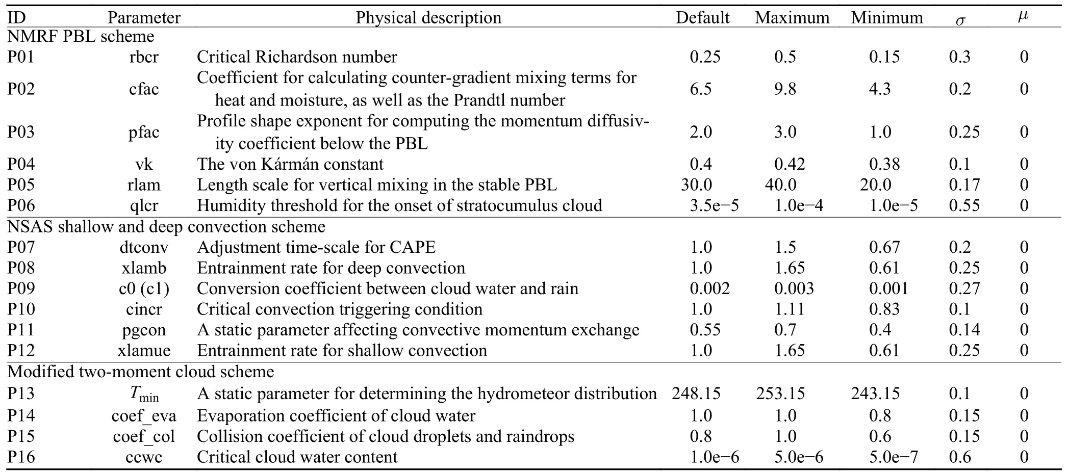
Table 1. The chosen parameters or variables in the SPP scheme developed for CMA-GEPS, along with their default, maximum, and minimum values, as well as the means (μ) and standard deviations (σ) of the stochastic perturbation patterns applied to these selected parameters or variables
To create a good error–spread relationship, the spatial and temporal correlation scales of the stochastic perturbation field Ψjhave been tuned by performing a series of sensitivity experiments with different correlation scales.It is found that larger spatial and temporal correlation scales will generate more ensemble spread. Therefore,for all chosen parameters or variables, the stochastic perturbations described in spectral space are characterized by a temporal correlation of 72 h and spatial correlation of a maximum truncation wavenumber-5 that corresponds to a large spatial correlation scale. These configurations are similar to those described in Ollinaho et al.(2017).
2.3 Numerical experiments
For investigating the impacts of SPP on CMA-GEPS comprehensively, five ensemble experiments (see Table 2) were conducted in this study. In the first two experiments (i.e., SPP_only and SPPT_only), the SPP and SPPT schemes were used separately, and the SVs-based IPs were disabled in order to reveal the underlying difference between the SPP and SPPT schemes from the viewpoint of the perturbation structure. The other three ensemble experiments with IPs were performed in order to benchmark the impacts of the SPP scheme on CMAGEPS by employing (1) IPs only (IPs_only), (2) IPs and the SPP scheme (IPs_SPP), and (3) IPs and the SPPT scheme (IPs_SPPT). The same set of SVs-based IPs were adopted by these three experiments. Therefore, the influences of the two stochastic schemes could be assessed and contrasted with the IPs_only, IPs_SPP, and IPs_SPPT experiments.
Moreover, all of the five experiments in Table 2 were conducted by using the 31-member CMA-GEPS (1 unperturbed control member and 30 perturbed members)with a resolution of 0.5° × 0.5° and forecast range of 15 days. The experimental period was chosen to cover one 10-day boreal warm period (i.e., 6–15 May 2019) as well as one 10-day boreal cold period (i.e., 1–10 December 2017). In the setup of each experiment, ensemble forecasts were initialized at 1200 UTC during the experimental period, which amounted to 20 start dates in total.
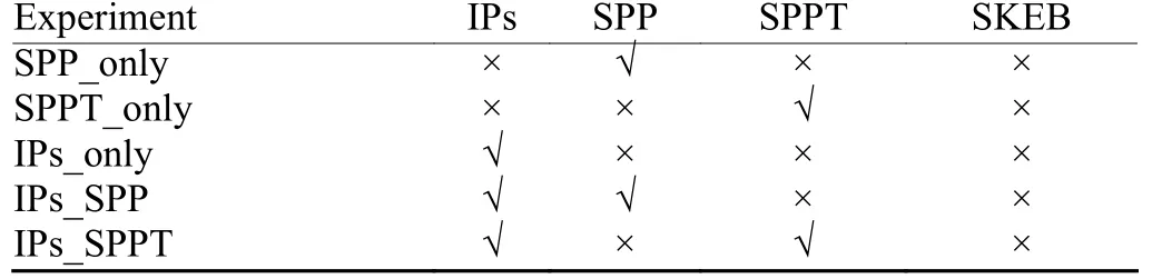
Table 2. Experiment configurations in this study (“×” denotes that the corresponding scheme is switched off, and “√” indicates that the corresponding scheme is turned on)
3. Perturbation structure
3.1 Physical tendency perturbation
Representations of model uncertainties through stochastic physics schemes contribute to diversity among ensemble members by changing physical tendencies of model forecast variables at each time step during the model integration. Hence, to illustrate the difference between the SPP and SPPT schemes in representing model uncertainties, tendencies from physical parameterizations accumulated in short-range forecasts were firstly compared between the SPP_only and SPPT_only experiments at the initialization time of 1200 UTC 8 May 2019.Owing to the inactive IPs in the experiments of SPPT_only and SPP_only, the difference between the tendencies could be attributed to the representation of model uncertainties in different approaches. Also, the 3-h accumulated physical tendencies on model levels were used for comparisons. Figure 1 shows the ensemble spread of the first 3-h accumulated tendencies for zonal wind, temperature, and specific humidity on different model levels. In the 0–3-h forecasts, the two schemes of SPP (red dashed lines) and SPPT (blue dashed lines)yield similar vertical distributions of tendency spread in the tropics (20°S–20°N) for the three examined model variables (Figs. 1a, d, g). However, the spread from SPP is greater than that from SPPT in the PBL (approxim-ately below model level 13), especially for temperature and specific humidity. In the Southern Hemisphere (SH;south of 20°S) and Northern Hemisphere (NH; north of 20°N), a clear difference between the two stochastic schemes can be observed. Generally, SPP produces larger tendency spread for temperature and specific humidity than SPPT in the lower PBL (approximately below model level 12); however, from the upper PBL to the upper troposphere (below model level 40), SPPT generates larger spread than SPP (Figs. 1e, f, h, i). For zonal wind,there is a small difference between the tendency spread(Figs. 1b, c). Overall, SPP can generate more tendency diversity than SPPT, mainly in the lower PBL, which may be explained by the tapered tendency perturbation magnitudes in the PBL. In the subsequent 21–24 hours of forecasts, SPP generally produces smaller tendency spread than SPPT in both the PBL and free troposphere(approximately below model level 45; red solid lines for SPP and blue solid lines for SPPT in Fig. 1), which is more visible for temperature in all three regions, as well as zonal wind and specific humidity in the SH and NH.Although SPPT does not introduce perturbations in the lower PBL directly, due to the use of the tapering function in the vertical direction, perturbations from the free troposphere would propagate downwards and contribute to variations in the PBL as the model integration proceeds. Therefore, in the following 21–24 hours of forecasts, the tendency spread (especially for temperature and humidity) from SPPT in the PBL turns to be comparable with, or even greater than, that from SPP.
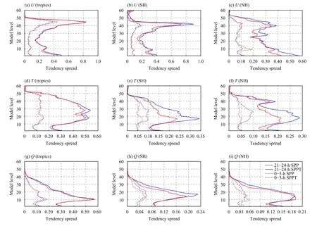
Fig. 1. Vertical profiles of ensemble spread for the 0–3-h (red dashed lines for SPP; blue dashed lines for SPPT) and 21–24-h (red solid lines for SPP; blue solid lines for SPPT) accumulated physical tendencies for (a–c) zonal wind [U; m s-1 (3 h)-1], (d–f) temperature [T; K (3 h)-1], and(g–i) specific humidity [Q; g kg-1 (3 h)-1], averaged over (a, d, g) the tropics, (b, e, h) SH, and (c, f, i) NH. The y-axis represents the model level,of which levels 9, 26, 40, and 49 are approximately equal to 950, 500, 200, and 100 hPa, respectively. Ensemble forecasts initialized at 1200 UTC 8 May 2019 were used to calculate the tendency spread.
The results about the physical tendency spread reveal that different perturbation structures are introduced by the SPP and SPPT schemes, and in the initial (0–3 h)forecast stage, the obvious difference between tendency spreads observed in the lower PBL is most likely caused by the different treatment of perturbations in the PBL.This also reflects the various nature of the two approaches in representing model uncertainties.
3.2 Total energy of perturbations
To further investigate the growth and evolution of perturbations generated by the two schemes, the difference in total energy (DTE; Zhang et al., 2003) is applied. The formula for DTE is as follows:
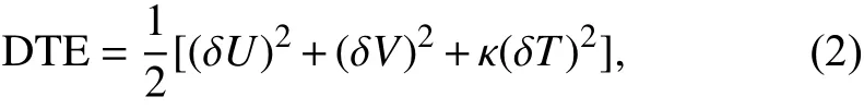
where δ denotes the difference between the perturbed and unperturbed (i.e., control) forecasts;U,V, andTrepresent the zonal wind, meridional wind, and temperature fields, respectively; and κ is a constant equal toin whichcpis the heat capacity of dry air at constant pressure (1004 J kg-1K-1) andTris the reference temperature (280 K). For each experiment described in Section 2.3, DTE was calculated and averaged over all perturbed members from all 20 initialization dates, which consisted of 10 days from 1200 UTC 6 to 15 May 2019 as well as 10 days from 1200 UTC 1 to 10 December 2017.
Figure 2 displays the vertical profiles of DTE averaged in the tropics, SH, and NH at different lead times(24, 96, 168, and 240 h) for experiments SPP_only (red dashed lines) and SPPT_only (blue dashed lines), in which IPs are not incorporated. It can be detected that the DTE of both experiments grows with the forecast lead time for all three regions, but with SPPT_only usually possessing a larger DTE than SPP_only, and the difference between SPP_only and SPPT_only being more evident in the SH and NH than in the tropics (note the differentx-axes). Moreover, the vertical distributions of DTE between the two experiments display similar features; that is, the peak values mainly emerge in the upper troposphere (300–150 hPa), which is probably associated with the strong dynamical instabilities around the upper-level jet. Feng et al. (2020) demonstrated that the fastest forecast error growth rate for wind and temperature is located near the upper-level jet (around 250 hPa),and this may lead to the fastest growth of perturbations in the upper troposphere, thus leading to the greatest DTE values.
Different features about DTE can be seen among the experiments of IPs_only, IPs_SPP, and IPs_SPPT, in which IPs are included. In Fig. 2, the DTE difference between experiments with (IPs_SPP: red solid lines;IPs_SPPT: blue solid lines) and without (IPs_only: black solid lines) stochastic physics is more noticeable in the tropics than in the SH and NH. In the SH and NH, the DTE values from the above three experiments are nearly the same. By comparing the DTE values of experiments with and without IPs in the extratropics, for example,IPs_SPP (red solid lines) and SPP_only (red dashed lines), it is clear that the SVs-based IPs play a dominant role, and make the greatest contribution to the growth of DTE in the SH and NH. Accordingly, the quite small difference in DTE among IPs_only, IPs_SPP, and IPs_SPPT is found in the extratropical areas. In the current version of CMA-GEPS, SVs are not calculated for the whole tropical region and they are computed only for up to six areas in the vicinity of tropical cyclones observed in the Northwest Pacific Ocean (Huo et al., 2020).When the computations of SVs for the tropics are activated, the generated IPs are localized and concentrated around (up to six) tropical cyclone systems; otherwise,there are few IPs in tropics. Therefore, the roles of SPP and SPPT are more prominent in the tropics when they are employed in combination with IPs. Furthermore, the additional DTE from IPs_SPP and IPs_SPPT relative to IPs_only in the tropics is more obvious in the middle and upper troposphere (Figs. 2a, d, g, j). In the first 96 h,IPs_SPPT generally has larger DTE than IPs_SPP (Figs.2a, d); nevertheless, in the following lead times (i.e., 168 and 240 h), IPs_SPP possesses a larger DTE, especially in the 300–150-hPa pressure levels, although SPP_only generates smaller DTE than SPPT_only at these lead times (Figs. 2g, j). This reflects the complex nonlinear interactions between model stochastic perturbations and IPs.
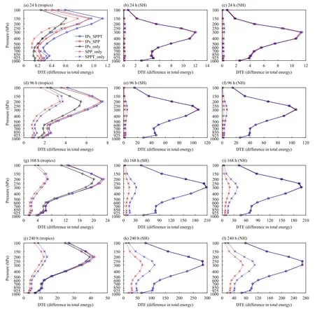
Fig. 2. Vertical profiles of area-weighted DTE (difference in total energy; m2 s-2) averaged in the tropics (left column), SH (middle column),and NH (right column) at the lead times of (a–c) 24 h, (d–f) 96 h, (g–i) 168 h, and (j–l) 240 h, for the five experiments of SPP_only (red dashed lines), SPPT_only (blue dashed lines), IPs_only (black solid lines), IPs_SPP (red solid lines), and IPs_SPPT (blue solid lines). The DTE was calculated from ensemble forecasts started on 20 dates covering one 10-day boreal warm period (1200 UTC 6–15 May 2019) and one 10-day boreal cold period (1200 UTC 1–10 December 2017).
4. Impacts on ensemble forecasts
In an EPS, stochastic physics schemes are utilized together with IP techniques so as to obtain a preferable match (i.e., a one-to-one ratio) between the ensemble spread and error of the ensemble mean. Consequently,based on the experiments using IPs, this section evaluates the impacts of the SPP scheme on the performances of CMA-GEPS by comparing the IPs_SPP and IPs_SPPT experiments with the IPs_only experiment. A range of verification metrics were applied to assess the performance of CMA-GEPS, including the ensemble mean rootmean-square error (RMSE), ensemble spread, outliers,and continuously ranked probability score (CRPS). These metrics were computed against the CMA-GFS analysis fields. In addition, precipitation skills in China were evaluated by computing the Brier score against observations at more than 2400 synoptic stations.
4.1 Ensemble spread and ensemble mean RMSE
For a statistically reliable ensemble, the ratio between the ensemble spread and RMSE of the ensemble mean should be one-to-one. Previous studies have reported that CMA-GEPS suffers from the under-dispersion problem(i.e., ensemble spread smaller than RMSE), particularly in the tropics (Li et al., 2019; Peng et al., 2019). Figure 3 depicts vertical distributions of the ensemble spread difference for zonal wind and temperature in IPs_SPP and IPs_SPPT relative to IPs_only. Considering the little difference in perturbation energy (i.e., DTE) between experiments IPs_SPP (IPs_SPPT) and IPs_only in the extratropics, it is unsurprising that the additional use of SPP(SPPT) does not create more spread in the SH and NH(Figs. 2, 3). In the tropics, both SPP and SPPT lead to obvious increases in ensemble spread, consistent with the result that the DTE increases of IPs_SPP and IPs_SPPT relative to IPs_only are mainly located in the tropics. Besides, larger spread increments appear above 300 hPa for zonal wind and in both the lower- and upper-level troposphere (approximately below 700 hPa and above 300 hPa) for temperature, which might arise from the dynamical instabilities at different levels. Furthermore, the spread increases from SPPT are generally larger than those from SPP in the short-range (48 h) forecasts, and then turn to be smaller than those from SPP in the mediumrange (144 h) forecasts. These results are in line with the DTE difference between IPs_SPP and IPs_SPPT summarized in Section 3.2. For an EPS, the measure of DTE is inferred to be a good indicator of ensemble spread,with greater magnitudes of DTE corresponding to more spread.
In terms of ensemble mean RMSE, the difference between IPs_SPP (IPs_SPPT) and IPs_only is smaller than that of ensemble spread (Figs. 3, 4). As revealed by Fig. 4, the RMSE is almost unchanged, or ameliorated slightly, due to the use of SPP or SPPT, except that SPPT leads to a slight increase in the RMSE of upper-level temperature in the tropics (Figs. 4g, h). This RMSE increase from the SPPT scheme may be caused by applying the same perturbation pattern to tendencies from radiation processes, regardless of whether it is clear-sky or cloudy-sky conditions (Leutbecher et al., 2017). To acquire a more physically consistent description of model uncertainty around the globe, Lock et al. (2019) revised the SPPT scheme in the ECWMF ensemble by not perturbing radiation tendencies from clear-sky processes,and thus made improvements in the ensemble spread–error relationship. Inspired by this study, we will test similar revisions to the radiation tendency perturbations in our SPPT scheme in the future.
To clarify the impacts of SPP and SPPT on the ensemble spread and RMSE from the domain-average viewpoint, the difference in ensemble spread and RMSE within the entire forecast range is presented in Fig. 5.Given the small impacts of SPP and SPPT in the NH and SH (as shown in Figs. 3, 4), Fig. 5 only presents the results in the tropics. Besides the representative upper-air forecast variables—namely, 850- and 200-hPa zonal wind, 850- and 200-hPa temperature, and 925- and 700-hPa specific humidity—surface variables such as 10-m zonal wind, 2-m temperature, and 2-m specific humidity were also evaluated. To determine the significance of the difference between experiments, a Student’st-test was applied at the 95% confidence level (also employed for the differences concerning other scores in the following analysis). It can be seen that the spread increases due to the use of SPP are statistically significant up to forecast day 15 for all examined surface variables (Figs. 5c, f, i),as well some of the upper-air variables, such as 850-hPa temperature and 700-hPa humidity (Figs. 5d, h), and up to days 8 or 11 for the other investigated variables (Figs.5a, b, e, g). The spread increases due to the application of SPPT generally hold at the 95% confidence level for forecasts shorter than day 10 (Fig. 5). In addition, for upper-level (200 hPa) temperature and lower-level (925 hPa) humidity, the SPP scheme yields more spread than SPPT in the whole forecast window (Figs. 5e, g). For example, on forecast day 6, compared against the reference experiment, IPs_only, the spread of 200-hPa temperature(925-hPa specific humidity) is increased by 18.3%(10.9%) for IPs_SPP and 13.7% (8.5%) for IPs_SPPT.With respect to the other examined variables, the spread increments generated by SPPT are greater in the short forecast range; however, these increments decline gradually with forecast lead time, and become comparable with, or smaller than, SPP at lead times beyond day 7(Figs. 5a, b, c, d, f, h, i). The RMSE difference is quite small, and does not pass the significance test at the 95%confidence level.
4.2 Outliers
Outliers, which are calculated as the frequency that the“truth” (or “analysis”) falls out of ensemble members(Wang et al., 2014), were also applied to illustrate the impacts of stochastic schemes on the forecast reliability.As exhibited in Fig. 6, a negative (positive) outlier difference between experiments denotes improved (deteriorated) reliability generated by SPP or SPPT. It is shown that, in the tropics, both schemes result in remarkable reductions of outliers (negative difference in Fig. 6). Also,the improvements in outliers from SPP are statistically significant in the entire forecast period for 850-hPa and 2-m temperature, as well as the three inspected humidity variables (Figs. 6d, f, g, h, i), and up to around day 12 for the remaining examined variables (Figs. 6a, b, c, e). Generally, the lead times at which the improvements from SPPT reach statistical significance are shorter than those from SPP. Besides, when compared against SPPT, SPP exhibits more improvements for 200-hPa temperature, 2-m temperature, 925-hPa specific humidity, and 2-m specific humidity during the whole forecast length (Figs. 6e,f, g, i). Taking 2-m temperature as an example, on forecast day 6, the outlier with SPP is 2.8% less than that with SPPT. For the other variables, SPPT usually performs better in the first 7-day forecasts, and then SPP behaves comparably, or even better than, SPPT in the following forecasts (Figs. 6a, b, c, d, h). For instance, the outlier of 200-hPa zonal wind for SPP is 1.3% more than that for SPPT on day 3, and 0.5% less than that for SPPT on day 8. In the NH and SH, both SPP and SPPT contribute to slight and similar reductions in outliers (figures omitted). These results are consistent with those from the ensemble spread.
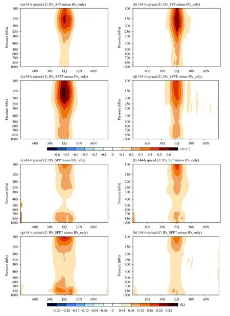
Fig. 3. Vertical profiles of differences in ensemble spread for the 48-h (left column) and 144-h (right column) forecasts of (a–d) zonal wind (U;m s-1) and (e–h) temperature (T; K) between experiments with and without stochastic physics schemes: (a, b, e, f) IPs_SPP relative to IPs_only(first and third rows); (c, d, g, h) IPs_SPPT relative to IPs_only (second and fourth rows). The spread differences were calculated from ensemble forecasts started on 20 dates covering one 10-day boreal warm period (1200 UTC 6–15 May 2019) and one 10-day boreal cold period (1200 UTC 1–10 December 2017).
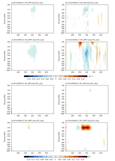
Fig. 4. As in Fig. 3, but for the ensemble mean RMSE.

Fig. 5. Differences in ensemble spread (dashed lines) and ensemble mean RMSE (solid lines) as a function of forecast lead time between experiments with and without stochastic physics schemes: (a–c) 850-hPa, 200-hPa, and 10-m zonal wind (U850, U200, and U10m; m s-1); (d–f) 850-hPa, 200-hPa, and 2-m temperature (T850, T200, and T2m; K); and (g–i) 925-hPa, 700-hPa, and 2-m specific humidity (Q925, Q700, and Q2m;g kg-1), averaged in the tropics for experiments IPs_SPP (red lines) and IPs_SPPT (blue lines) relative to IPs_only (i.e., IPs_SPP minus IPs_only,and IPs_SPPT minus IPs_only). Statistical significance of increases (decreases) in spread (RMSE) at the 95% confidence level is highlighted with circles (crosses) by applying a Student’s t-test. The differences were calculated from ensemble forecasts started on 20 dates covering one 10-day boreal warm period (1200 UTC 6–15 May 2019) and one 10-day boreal cold period (1200 UTC 1–10 December 2017).
4.3 CRPS
Impacts of SPP and SPPT on the probabilistic forecast skills of CMA-GEPS were assessed by CRPS, which measures the difference between the observed and forecasted cumulative distribution functions (Hersbach,2000). This metric is a negatively oriented score, with smaller values denoting better probabilistic skills. Figure 7 illustrates the CRPS difference from the IPs_SPP and IPs_SPPT experiments against the IPs_only experiment in the tropics, in which the greater negative values of the CRPS difference stand for more improvements in probabilistic skill. For all variables except 200-hPa temperature, both SPP and SPPT enhance the probabilistic forecast skill (negative difference in Figs. 7a, b, c, d, f, g, h,i). In terms of 200-hPa temperature, SPPT induces a degraded forecast skill (but not significant) associated with the increase in ensemble mean RMSE (Figs. 7e, 5e),which can presumably be attributed to the improper treatment of tendencies from clear- and cloudy-sky radiation.Leutbecher et al. (2017) pointed out that, compared with tendencies from cloudy-sky radiation, those from clearsky radiation should be more certain. In the current SPPT scheme, the two types of tendencies are perturbed in the same way, and assume to possess the same degree of uncertainty. However, the SPP scheme still causes an improved skill (negative difference in Fig. 7e), and this improvement is statistically significant in the first 8-day forecasts. The majority of the CRPS improvements for specific humidity are statistically significant, which does not hold for temperature and zonal wind. By comparing SPP against SPPT, it can be seen that SPP displays overall better probabilistic skills for 200-hPa temperature, 2-m temperature, 925-hPa specific humidity, and 2-m specific humidity (Figs. 7e, f, g, i). For example, on forecast day 6, compared to the reference experiment, IPs_only,the CRPS of 925-hPa specific humidity is improved by 4.5% for IPs_SPP, and by 3.8% for IPs_SPPT. Regarding the other inspected variables, the skills of SPPT are higher at the shorter lead times, and then exhibit comparable skills with SPP at the longer lead times (approximately beyond forecast day 7; Figs. 7a, b, c, d, h). In the NH and SH, little difference in CRPS appears between IPs_only, IPs_SPP, and IPs_SPPT (figures omitted).
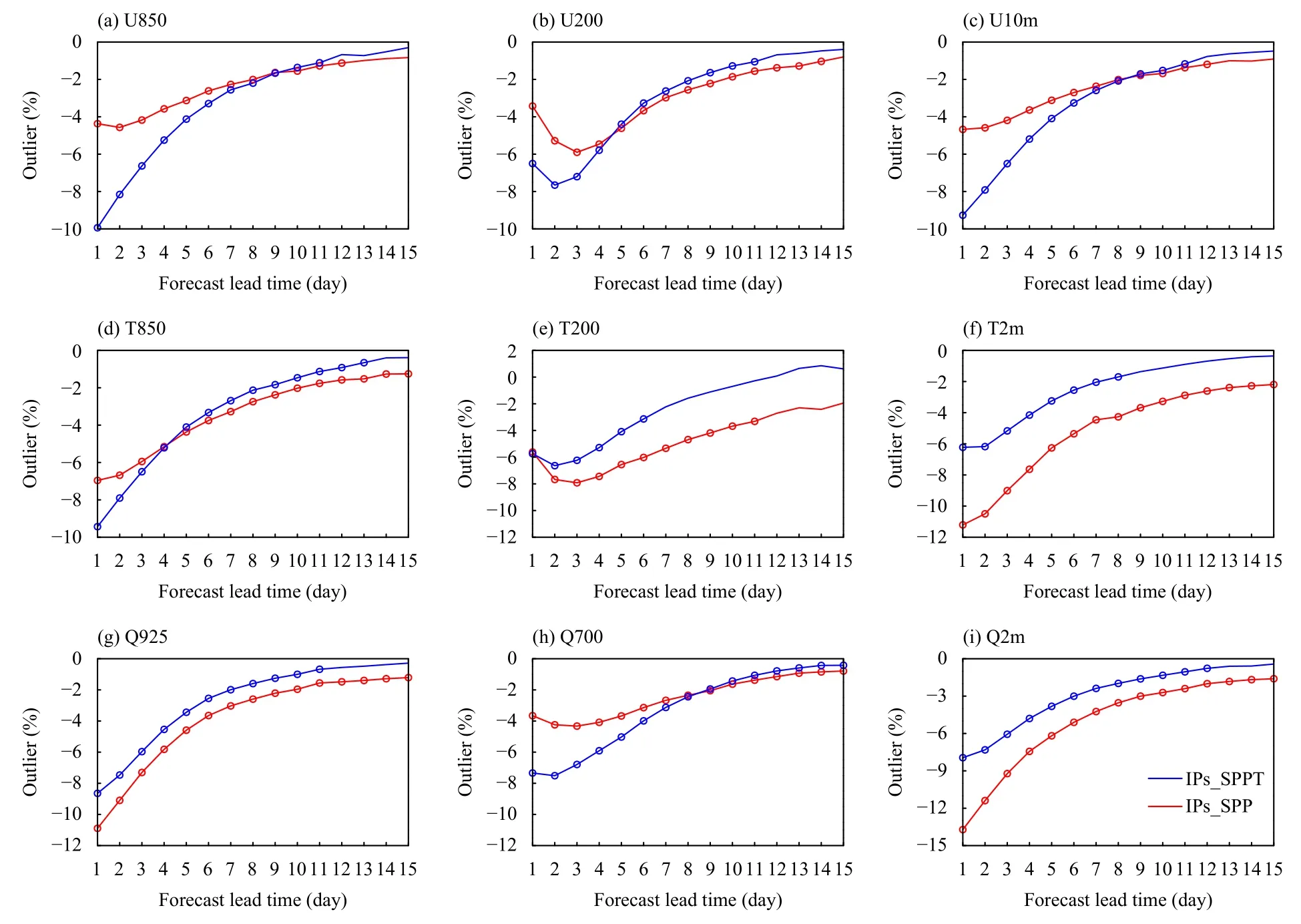
Fig. 6. As in Fig. 5, but for outliers (%).
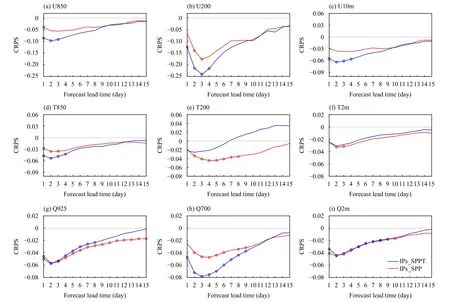
Fig. 7. As in Fig. 5, but for CRPS.
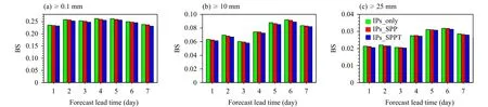
Fig. 8. Brier scores (BS) of 24-h accumulated precipitation that exceeds (a) 0.1 mm (light rain), (b) 10 mm (moderate rain), and (c) 25 mm(heavy rain) in China for the different ensemble experiments of IPs_only (green bars), IPs_SPP (red bars), and IPs_SPPT (blue bars). The scores were calculated from ensemble forecasts started on 10 dates covering a 10-day boreal warm period (1200 UTC 6–15 May 2019).
4.4 Precipitation verification
Influences of the stochastic schemes on precipitation forecasts in China were assessed by performing verifications against observations from over 2400 synoptic stations provided by the National Meteorological Information Centre of the CMA. Considering the lack of precipitation in the boreal cold period of 1–10 December 2017,only forecasts in the boreal warm period of 6–15 May 2019 are compared in this section. To reasonably reflect the predictability of precipitation in global ensembles,only 1–7-day forecast skills were evaluated. Figure 8 gives the Brier scores (Brier, 1950) of 24-h accumulated precipitation in the three experiments of IPs_only,IPs_SPP, and IPs_SPPT, for three thresholds (light rain:[0.1, 10 mm); moderate rain: [10, 25 mm); heavy rain:[25, 50 mm)). The smaller the Brier scores, the better the precipitation probabilistic skill. Compared with only using IPs, the inclusion of the SPP and SPPT schemes improves the skill for light rain and moderate rain to some extent, and SPPT shows slightly better skill than SPP.The Brier score difference for IPs_SPP and IPs_SPPT relative to IPs_only does not pass the significance test,which may be associated with the limited frequency of precipitation events in the selected experimental period.
5. Discussion
When the SVs-based IPs are employed, the implementation of SPP mainly improves the ensemble spread in the tropics. Due to the relatively large number of parameters or variables (16 in total) perturbed by the SPP scheme, as well as the complex interactions between the perturbed quantities, it is difficult to clarify which parameter or variable perturbation is more crucial in generating the ensemble spread (i.e., the forecast uncertainty). In practice, impacts of perturbations from different parameterization schemes are also worthy of investigation. Preliminary comparisons have been made between the three ensembles constructed by only perturbing the quantities in the PBL scheme, the convection scheme, and the cloud scheme, respectively. It has been found that perturbations from the convection scheme and the PBL scheme play a more important role in generating ensemble spread. Both SPP and SPPT show minor impacts in the extratropics. One of the primary reasons is the dominant influence of the SVs-based IPs in extratropics. If the magnitudes of IPs are reduced to some extent, the impacts of the two schemes may be pronounced, but more testing is needed to prove this. Another reason may lie in the moderate perturbation magnitudes used in SPPT or SPP, limited by the computational stability.
From the current results, the SPP scheme displays some advantages over the SPPT scheme in improving the ensemble performance of CMA-GEPS; in particular, by performing better in improving forecasts for the mediumrange (approximately beyond day 7) lead times. Meanwhile, in terms of the 1–7-day forecast performance, SPP adds fewer benefits than SPPT. Thus, work to optimize the current SPP scheme is still needed, and one direction is to improve and increase the selections of key parameters. For example, sensitive parameters associated with land surface processes can be further perturbed to add to the benefits of the SPP scheme.
6. Conclusions
In this study, the SPP scheme has been developed for CMA-GEPS in order to represent model uncertainties at physical process levels by perturbing 16 crucial parameters or variables chosen from three parameterization schemes—for the PBL, cumulus convection, and cloud microphysics. Temporally and spatially correlated perturbations satisfying the log-normal distributions are applied to these selected parameters or variables, and each parameter or variable is perturbed independently. With the SPPT scheme as a baseline for comparison, a comprehensive analysis of how the SPP scheme influences the performance of CMA-GEPS is implemented from the perspective of perturbation characteristics and ensemble performance. To achieve this, two groups of ensemble experiments have been carried out, between which the difference lies in whether IPs are activated. One group does not include IPs and only uses stochastic physics(i.e., the SPP_only and SPPT_only experiments), while the other group employs the SV-based IPs and includes the optional use of stochastic schemes (i.e., the IPs_only,IPs_SPP, and IPs_SPPT experiments).
The difference between the ensemble spread of physical tendencies in short-range (i.e., 0–3 and 21–24 h)forecasts from the SPP_only and SPPT_only experiments suggests that the SPP and SPPT schemes can tackle different aspects of model uncertainties, and the SPP scheme is more favorable in representing uncertainty from the PBL. Moreover, in view of the growth and evolution of perturbations caused by the separate use of SPP and SPPT, when there are no IPs, the vertical profiles of DTE from SPP and SPPT are similar in all three regions (the tropics, SH, and NH), showing that the DTE is increased with the forecast lead time and the peak values mainly appear in the upper troposphere due to the strong dynamical instabilities around the upper-level jet.However, the magnitudes of DTE from SPPT are larger than those from SPP, especially in the SH and NH. When the IPs are employed together, the DTE arising from SPP and SPPT exhibits a different performance. In the SH and NH, both SPP and SPPT have few impacts on DTE due to the dominant role of IPs, which are calculated from SVs. However, obvious increases in DTE are induced by the two schemes in the tropics. In the first few forecast days, the DTE increases from SPP are generally smaller than those from SPPT, and then larger increases come from SPP approximately beyond day 7. The above results indicate that there are complex nonlinear interactions between model stochastic perturbations and IPs.
Relative to using IPs alone, the inclusion of SPP improves the performance of CMA-GEPS mainly in the tropics, consistent with the earlier results that increases in DTE introduced by SPP are primarily located in the tropics when IPs are applied. In addition, the introduction of SPP contributes to a more reliable ensemble by increasing the spread and reducing outliers; and the vast majority of the spread increases and outlier reductions are significant at the 95% confidence level. Moreover, the SPP scheme helps to reduce the CRPS scores, and thus plays a positive role in improving the probabilistic skill. Only the CRPS improvements for 925-hPa, 700-hPa, 2-m specific humidity, and 200-hPa temperature reach statistical significance for the majority of forecast lead times. The precipitation skill for light rain and moderate rain in China can also be improved by SPP to some extent.
Comparisons concerning the impacts on forecast performance were also made between SPP and SPPT when used together with IPs, respectively. For 200-hPa and 2-m temperature, along with 925-hPa and 2-m specific humidity, SPP usually shows more improvements in both ensemble reliability and probabilistic forecast skill during the whole forecast range. For other investigated variables, at shorter lead times, SPPT contributes to more reliable and skillful ensembles; however, at lead times approximately beyond day 7, SPP leads to more improvements in ensemble reliability and exhibits probabilistic skills similar to SPPT. For a global medium-range (3–15 days) EPS, the improvements for longer than day 7 are still important. Therefore, the two methods have their own merits.
This study has illustrated the potential value of the SPP scheme in CMA-GEPS. Currently, research on the combined use of SPP and SPPT has been explored in limited-area EPSs, and some advantages have been reported (Wastl et al., 2019; Xu et al., 2020). Similar strategies can also be introduced into global ensembles.For example, the insufficient perturbations in the PBL for the SPPT scheme can be compensated for by perturbing key parameters in the parameterization of the PBL.
Acknowledgments.The authors are extremely grateful to the reviewers and editors for their helpful comments and suggestions.
 Journal of Meteorological Research2022年5期
- Journal of Meteorological Research的其它文章
- Assessing 10 Satellite Precipitation Products in Capturing the July 2021 Extreme Heavy Rain in Henan, China
- Refined Evaluation of Satellite Precipitation Products against Rain Gauge Observations along the Sichuan–Tibet Railway
- Direct Radiative Effects of Dust Aerosols over Northwest China Revealed by Satellite-Derived Aerosol Three-Dimensional Distribution
- Assimilation of All-Sky Radiance from the FY-3 MWHS-2 with the Yinhe 4D-Var System
- Interannual Relationship between Summer North Atlantic Oscillation and Subsequent November Precipitation Anomalies over Yunnan in Southwest China
- Intensified Impact of the Equatorial QBO in August–September on the Northern Stratospheric Polar Vortex in December–January since the Late 1990s