A bayesian optimisation methodology for the inverse derivation of viscoplasticity model constants in high strain-rate simulations

Shnnon Ryn ,Julin Berk ,Sntu Rn ,Brodie McDonld ,Sveth Venktesh

a Applied Artificial Intelligence Institute(A2I2),Deakin University,75 Pigdons Rd,Waurn Ponds,VIC,3216,Australia

b Defence Science and Technology Group,506 Lorimer Street,Fishermans Bend,VIC,3207,Australia

Keywords:Constitutive modelling Finite element Bayesian optimisation Finite element model updating

ABSTRACT We present an inverse methodology for deriving viscoplasticity constitutive model parameters for use in explicit finite element simulations of dynamic processes using functional experiments,i.e.,those which provide value beyond that of constitutive model development.The developed methodology utilises Bayesian optimisation to minimise the error between experimental measurements and numerical simulations performed in LS-DYNA.We demonstrate the optimisation methodology using high hardness armour steels across three types of experiments that induce a wide range of loading conditions:ballistic penetration,rod-on-anvil,and near-field blast deformation.By utilising such a broad range of conditions for the optimisation,the resulting constitutive model parameters are generalised,i.e.,applicable across the range of loading conditions encompassed the by those experiments(e.g.,stress states,plastic strain magnitudes,strain rates,etc.).Model constants identified using this methodology are demonstrated to provide a generalisable model with superior predictive accuracy than those derived from conventional mechanical characterisation experiments or optimised from a single experimental condition.

1.Introduction

In the numerical analysis of a highly dynamic impact event such as a ballistic penetrator impacting upon an armoured target,selection of a constitutive model and derivation of the model constants is a critically important step.A constitutive model should be selected such that it is it capable of capturing key deformation characteristics of the simulated material at the loading conditions of interest without being unnecessarily complex.Model constants are classically derived by direct fitting of the constitutive model to mechanical and,where necessary,shock characterisation data that covers the range of loading conditions to which the model will be applied,see e.g.,Ref.[1].More recently,inverse strategies are being employed which incorporate numerical simulation of the experiment and iterative adjustment of model constants until measured signals can be numerically reproduced,e.g.,Finite Element Model Updating(FEMU)[2],Constitutive Equation Gap Method(CEGM)[3],etc.A schematic representation of these strategies is provided in Fig.1.Inverse strategies permit the utilisation of more extensive data than that classically used,for example digital image correlation(DIC)for surface strain.As a result,these methods can enable the derivation of model constants with fewer experiments than the classical technique.Reviews of such inverse strategies are provided in,e.g.,Refs.[4,5].

Such inverse strategies are typically employed on thermomechanical tests,e.g.,uniaxial tension[7],cruciform[8],etc.A limited number of studies have investigated these methods applied to functional experiments,that is experiments which have utility beyond the derivation of constitutive model constants.For example,Walls et al.[10]performed inverse modelling to optimise parameters of energetic materials from experiments more typically used for model validation,i.e.,cylinder test and wedge test.Portone et al.[11]performed model identification and tuning of existing model constants based on inverse modelling of a penetration vs.time experiment.These approaches,however,may result in model constants which are not generalisable—that is,for experimental conditions different to those used in the inverse approach,the identified constants will be inaccurate.

In this study we apply Bayesian optimisation to perform constitutive model selection and derivation of model constantsfrom a range of functional experiments.These experiments provide a rich source of data which is often underutilised in numerical studies,i.e.,they are used only for the validation of simulation models.By including multiple experiments in the optimisation,representing a wide range of loading conditions and induced material responses,the resulting model should be better able to generalise to previously unseen conditions,provided that those conditions are within the range bounded by the initial experiments used for the optimisation.The proposed methodology provides the means to generate robust material models in a rapid and low-cost manner without the need for typical mechanical characterisation experiments.Rather,all the necessary experiments are useful in terms of the desired application,e.g.,blast protection,ballistic protection,etc.

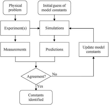
Fig.1.Schematic representation of inverse strategies such as FEMU which attempt to identify constitutive model constants by minimising the error between experimental measurements and numerical simulations of such experiments,after Ref.[6].

2.Experiments

2.1.Time-resolved ballistic penetration experiments

In Ref.[12]a series of ballistic experiments are conducted with 0.5 cm diameter,5.0 cm long cylindrical tungsten-alloy long rod penetrators against steel targets.The steel used in the experiments was a high-hardness armour grade(HzB-W),manufactured by Thyssen Stahl AG,Germany,with a density of 7.85 g/cm,a hardness of 440±20 Vickers,and a yield strength of 1.45±0.1 GPa.Two series’of nominally identical experiments were conducted in which a single radiograph was generated during each experiment at progressively later times.The data was collated to generate a quasi-time resolved penetration curve for the two experimental conditions,namely:a striking velocity of 1250 m/s against a 2.90 cm thick target,and a striking velocity of 1700 m/s against a 4.95 cm thick target.A schematic of the experiments is provided in Fig.2 along with a reproduction of the experimental results.The experimental uncertainty is reported in Ref.[12]to be±0.02 cm,however Portone et al.[11]suggest an uncertainty of approximately±0.06 cm is more suitable based on the inflection in the experimental data against the 2.90 cm thick target between 30 and 50 μs post-impact.The 2.90 cm target experiments are observed to exhibit more experimental uncertainty than the 4.95 cm thick target experiments,as indicated by the polynomial trend fit to the measurements.

2.2.Rod-on-anvil experiments

Ryan et al.[14]present the results of a series of rod-on-anvil experiments using a high-hardness armour(HHA)grade steel,conforming to MIL-DTL-46100 Class 1[15],with a nominal hardness of 500 Brinell(approximately 530 Vickers)and a nominal yield strength of 1.30 GPa.A series of eight experiments were conducted using the setup described in Ref.[16].Cylindrical steel rods of 6.35 mm diameter and 31.75 mm length were impacted on a rigid anvil at impact velocities between 148 m/s and 236 m/s.Transient deformation profiles of the rods were recorded using high-speed photography during the experiment,as well as surface strain measurements via digital image correlation(DIC).Post-test length,nose-diameter,and profile measurements were also recorded.A schematic of the experimental setup is provided in Fig.3 and the final rod length and nose diameter measurements are provided in Fig.4.For this study we select two experiments for utilisation in the hyperparameter optimisation that are below the velocity required for fracture initiation of the material:(1)impact velocity of 184 m/s,and(2)impact velocity of 208 m/s.

The HHA steel used for experiments in Ref.[14]is not the same as the HzB-W used in Ref.[12],however the nominal mechanical properties are similar.Furthermore,Anderson et al.using the model constants for Class 1 HHA in CTH,was able to closely match the experimental performance of the HzB-W steel.Thus,for the sake of this investigation we consider the two materials to be of a similar grade and thus expect a similar but not identical level of performance.

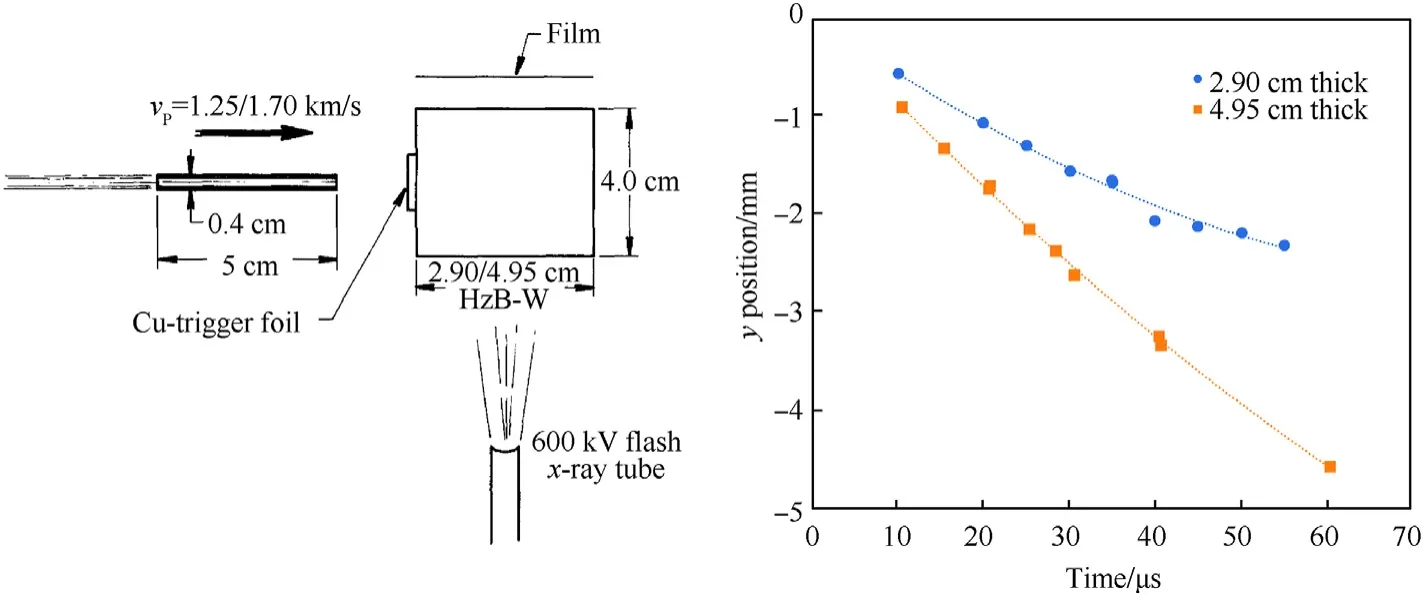
Fig.2.Long-rod ballistic penetration experiment from Ref.[12],setup(left)and results(right).A 2nd order polynomial fit has been added to each of the experimental data series.

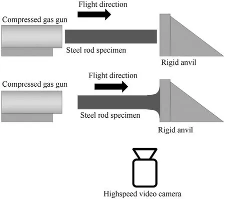
Fig.3.Schematic of the rod-on-anvil experiment from Ref.[14],after Ref.[16],where the rod is fired from a compressed gas gun into a rigid anvil and a highspeed video camera is used to record the transient deformation of the rod.Two image sequences are shown,an initial image where the rod is yet to impact the anvil,and a subsequent image where the rod has impacted the anvil and the nose has begun to deform.

2.3.Explosion bulge experiments

McDonald et al.[17]present the results of a series of near fieldblast experiments against four high strength steels,including a HHA steel conforming to MIL-DTL-46100 Class 1[15]with a nominal hardness of 500 Brinell(approximately 530 Vickers)and a nominal yield strength of 1.20 GPa.A total of 15 experiments were conducted against nominally 4.0 mm thick HHA plates at stand-off distances(SODs)of 13 mm and 25 mm between the closest edge of the cylindrical PE4 charges and the plate.The target plates were square,with a side length of 500 mm,and were clamped around the outer 50 mm of the plate,leaving a 400 mm×400 mm aperture(exposed area).The explosive charge had a diameter of 50 mm while the height(and subsequently mass)of the explosive charge was varied to determine a threshold at which the plate begun to rupture under the blast load.The experimental setup is shown in Fig.5 together with example deformation profiles from Ref.[17].For this study we select two experimental conditions for utilisation in the hyperparameter optimisation:(1)37.5 g explosive mass at 13 mm stand-off distance,and(2)57.5 g explosive mass at 25 mm stand-off distance.

3.Numerical simulations

All numerical simulations have been conducted in the explicit structural mechanics solver of LS-DYNA from LSTC.Four common constitutive models were evaluated:the semi-analytical,dislocation mechanics-based Zerilli-Armstrong(ZA)model[13];the phenomenological Johnson-Cook(JC)model[18];a modified variant of the Johnson-Cook(MJC)model that incorporates a two term Voce strain-hardening saturation response and a power-law formulation of strain rate hardening,after Ref.[19],and;another variant of the Johnson-Cook model,comparable to the MJC model with a two-part product description of strain rate hardening,after Ref.[14],referred to herein as TJC.The ZA and JC models are used with a Gruneisen equation-of-state(EoS),while the MJC,and TJC models use a linear EoS.

The ZA model is defined for a body centred cubic(BCC)as:

where σis the sum of the athermal,strain rate and temperature independent yield strength,σ(MPa),and the Hall-Petch grain strengthening relationship,kd,k is the micro-structural stress intensity(MPa mm);d is the average grain diameter(mm),ε is the plastic strain(mm/mm),˙ε is the plastic strain rate(s),T is the instantaneous temperature(K),and;C,C,C,C,and n are the empirical model constants(also referred to herein as optimisation hyperparameters).In practice σis often handled as an additional empirical constant,as done herein.

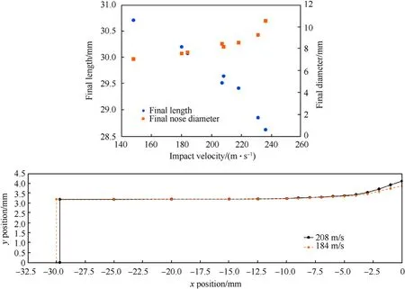
Fig.4.Results of the rod-on-anvil experiments for a HHA steel reported in Ref.[14],plotted in terms of;Top:final rod length(blue circle markers)and nose-diameter(orange square markers)vs.impact velocity,and;Bottom:rod profile viewed from the side,showing results for the 184 m/s and 208 m/s impact events.The y-position is averaged from the top and bottom measurements on the experimental image,the variation of which is represented by error bars.

Fig.5.Left:Blast experiment setup from Ref.[17].The explosive is located to the left of the target plate(left-most vertical plate)with the base of the cylindrical explosive parallel to the front surface of the plate.Right:Example permanent deformation profiles induced by the blast event and recorded via post-test 3D scanning.

The JC model is defined as:

where˙εis the reference strain rate(s)set equal to 1.0 in this study,Tis the reference temperature(K)set equal to 298 K in this study,Tis the melting temperature(K),and;A,B,n,C,and m are the empirical model constants.

The MJC model is defined as:

where A,B,n,Q,c,Q,c,β,and m are the empirical model constants.As per the JC model,the reference strain rate˙εis set equal to 1.0 sand the reference temperature Tis set equal to 298 K for this investigation.

The TJC model is defined as:

where A,B,n,Q,c,Q,c,β,β,and m are the empirical model constants.The reference plastic strain rates,˙εand˙ε,can also be considered empirical model constants,but should typically be defined in relation to the characterisation test conditions.As per the JC model,the reference temperature Tis set equal to 298 K for this investigation.

3.1.Time-resolved ballistic penetration simulations

The long-rod penetration experiments from Ref.[12]have been simulated in 2D axial-symmetry using four-node shell elements for the projectile and target parts.The geometry of the simulated projectile and target is nominally identical to that described in Section 2.1.Both the projectile and the target parts are meshed using quadrilateral elements with an edge length of 0.2 mm(in the target the element size is graded outside the penetration cavity)based on the findings of a mesh sensitivity study.The target was modelled as a cylinder with a radius of 36 mm and used a rigidly clamped boundary around the outer edge(i.e.,no rotation or translation).Contact was modelled using a two-way stiffness-based penalty formulation that incorporates Coulomb friction(for more details see the LS-DYNA theory manual[20]).The numerical setup is shown in Fig.6.

3.2.Rod-on-anvil simulations

The rod-on-anvil experiments were simulated in 3D using 8-node,reduced-integration(constant stress)hexahedral solid elements for the steel rod.The rod geometry is 6.35 mm in diameter and 31.75 mm in length,nominally identical to that described in Section 2.2.ALE smoothing and 2nd order advection was used to prevent numerical instabilities associated with misformed elements at the nose of the rod in all simulations except those using the TJC model,which cannot be used with ALE smoothing in LSDYNA.The anvil was modelled the*RIGIDWALL_PLANAR keyword in LS-DYNA which provides a simple means for treating contact between a rigid body and the nodal points of a deformable body.Frictionless sliding after contact was modelled for the interface between the rod and anvil.The numerical setup is shown in Fig.7.

3.3.Blast simulations

The blast simulations were simulated in 2D axial symmetry using a multi-material arbitrary Lagrange Eulerian(MMALE)approach.The target plate was modelled as a cylindrical plate with a thickness of 4 mm and a radius of 250 mm.The outer 50 mm of the plate was clamped between constrained elastic parts to mimic the experimental condition,leaving an exposed cylindrical surfacewith a 200 mm radius.Although varying from the experimental condition,in which a square plate was used(see Section 2.3),preliminary simulations found negligible influence in the simulated plate deformation between 2D axial symmetric simulations using a cylindrical plate and 3D quarter symmetry plates using a square plate.Thus,the 2D axial symmetric plate was used in order to reduce the computational time.

Fig.6.Numerical setup for the rod penetration simulation where the tungsten alloy rod(in pink)is travelling from the top to the bottom of the page and the left edge of the simulation represents the rotational axis of symmetry.The inset shows a zoomed in view of the mesh discretisation about the impact location.

Fig.7.Numerical setup for the rod-on-anvil simulation where the rod is moving from left to right in the top left image and impacts upon the rigid wall(transparent with border).ALE smoothing is used when possible to avoid excessive mesh distortion at the nose of the rod.

The expansion and interaction of the detonation product with the surrounding air was modelled within a Eulerian domain and transferred to the target plate via a penalty-based coupling algorithm.The target plate was meshed using quadrilateral,4-node shell elements with an edge length of 0.4 mm(i.e.,10 elements through the plate thickness).The detonation and expansion of the PE4 explosive charge was modelled using a high explosive burn material model and the Jones-Wilkens-Lee(JWL)equation of state.Model parameters for C4[21]were used,consistent with the approach in Ref.[22].The numerical setup is shown in Fig.8.In the simulations the explosive loading was complete within the first 0.05 ms post-detonation.At 1.0 ms post-detonation we applied nodal damping to the plate to damp out the elastic reverberations and measure the final deformation at 20 ms post detonation.An example of the nodal position(Y-axis,representing vertical movement)vs.time is plotted in Fig.8.The dissipation of the elastic reverberations is apparent by 20 ms post-detonation.

Fig.8.Top:Annotated setup of the 2D axial symmetric blast simulations.Bottom:vertical position measured on the rear surface of the plate along the axis of symmetry showing the initial loading phase followed by elastic rebound and reverberation which is artificially damped out by 20 ms post detonation via implementation of nodal damping.

4.Optimisation methodology

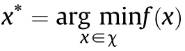
Our goal is to build numerical simulation models that employ constitutive models and constants,herein referred to as hyperparameters,which minimise the error between experimental measurements and simulation outputs.This will be achieved through an iterative process in which(1)a random initial guess of material hyperparameters is made(for a pre-defined constitutive model),x,(2)simulations are conducted with those hyperparameters,and(3)the results are compared with experimental measurements to determine the total simulation error.An optimisation function is tasked with modifying the hyperparameters and repeating this process until a minimum error is obtained,from which the optimal constitutive model hyperparameters can be identified.

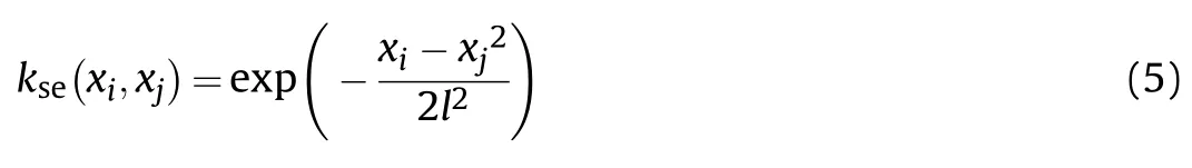
where l is a length scale parameter.This length scale is usually determined through maximum likelihood and is updated every few iterations.This is a very simple and effective kernel that produces relatively smooth function predictions and is hence robust to overfitting.However,some real-world systems may deviate from the square exponential kernel's strong smoothness assumptions.For more details on GP kernels we refer readers to Ref.[24].

A thorough review of Bayesian optimisation for adaptive experimental design is provided in Ref.[26].

4.1.Constitutive model selection

To identify the constitutive model which can best reproduce the material response observed in the experiments we run five different instances of Bayesian optimisation(BO)for each constitutive model option:ZA,JC,MJC,and TJC.Each instance is initiated with a batch of simulations that use random hyperparameter(model constant)sets chosen via a Latin hypercube method.The number of initial simulations performed corresponds to 3 times the dimensionality of the optimisation,e.g.,for the ZA model,which has 6 hyperparameters,there are 18 initial simulations conducted.The random hyperparameter selection is constrained to ensure a realistic stress-strain response.

·For ZA:σ?[0.0,3.0×10]Pa;C?[0.5×10,3.0×10]Pa;C?[0.0,1.0×10];C?[0.0,1.0×10];C?[0.0,3.0×10]Pa;and n?[0.01,1.5]

·For JC:A?[0.0,3.0×10]Pa;B?[0.0,3.0×10]Pa;n?[0.0,1.0];C?[0.0,0.1];m?[0.5,1.5]

·For MJC:A?[0.0,3.0×10]Pa;B?[0.0,3.0×10]Pa;n?[0.0,1.0];Q?[0.0,3.0×10]Pa;c?[0.0,2000];Q?[0.0,3.0×10]Pa;c?[0.0,2000];β?[0.0,0.1];m?[0.5,1.5]

·For TJC:A?[0.0,3.0×10]Pa;B?[0.0,3.0×10]Pa;n?[0.0,1.0];Q?[0.0,3.0×10]Pa;c?[0.0,2000];Q?[0.0,3.0×10]Pa;c?[0.0,2000];˙ε?[1.0×10,1.0]s;β?[0.0,0.1];˙ε?[1.0,1.0×10]s;β?[0.0,0.1],m?[0.5,1.5]

The results of the initial simulations provide the data required to generate the initial GP surrogate model,which is effectively a machine learning representation of the finite element simulation with input equal to the strength model hyperparameters and output equal to the simulation results(e.g.,penetration vs.time curve).

For the model selection step all six experiments are used to conduct the optimisation,namely:

1)Experiment 1:Penetration vs.time(projectile nose position)for impact at 1250 m/s against the 2.90 cm thick target,measured at 10.0 μs,19.9 μs,24.9 μs,30.0 μs,34.9 μs,39.9 μs,44.9 μs,50.0 μs,55.0 μs post-impact

2)Experiment 2:Penetration vs.time(projectile nose position)for impact at 1700 m/s against the 4.95 cm thick target,measured at 10.4 μs,15.3 μs,20.5 μs,25.3 μs,28.3 μs,30.5 μs,40.4 μs,60.3 μs post-impact

3)Experiment 3:Final deformed rod profile(y-position)following impact at 184 m/s,measured at 0 mm,1 mm,2 mm,3 mm,4 mm,5 mm,6 mm,7 mm,8 mm,9 mm,10 mm,12.5 mm,15 mm,20 mm,and 25 mm from the nose

4)Experiment 4:Final deformed rod profile(y-position)following impact at 208 m/s,measured at 0 mm,1 mm,2 mm,3 mm,4 mm,5 mm,6 mm,7 mm,8 mm,9 mm,10 mm,12.5 mm,15 mm,20 mm,and 25 mm from the nose

5)Experiment 5:Final deformed rod profile(y-position)following detonation of a 37.5 g explosive at 13 mm stand-off distance,measured at 0 mm,5 mm,10 mm,15 mm,20 mm,30 mm,40 mm,50 mm,60 mm,70 mm,80 mm,100 mm,120 mm,140 mm,160 mm,180 mm,and 200 mm along the radial span from the axis of symmetry

6)Experiment 6:Final deformed rod profile(y-position)following detonation of a 57.5 g explosive at 25 mm stand-off distance,measured at 0 mm,5 mm,10 mm,15 mm,20 mm,30 mm,40 mm,50 mm,60 mm,70 mm,80 mm,100 mm,120 mm,140 mm,160 mm,180 mm,and 200 mm along the radial span from the axis of symmetry

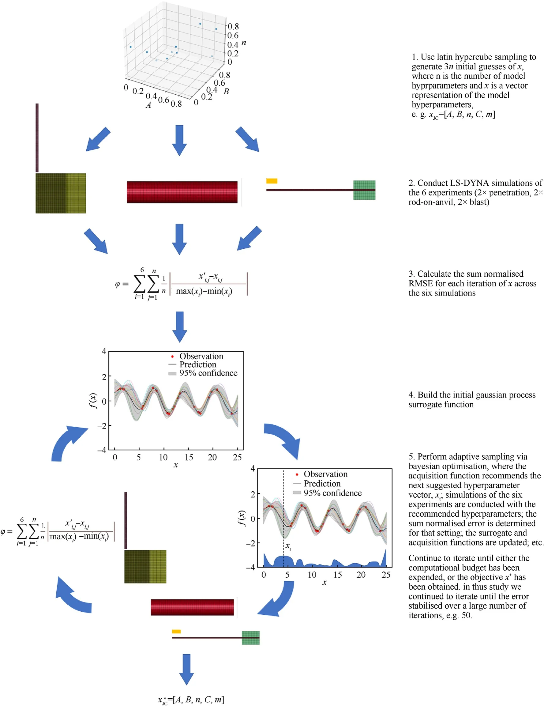
Fig.9.Schematic of the BO process applied in this study.Lower dimensional representations of the Latin hypercube and GPs are provided for visualisation,the actual dimensionality is defined by the number of hyperparameters in the viscoplastic constitutive model.

The result of the initial optimisation runs for each of the constitutive model options are given in Table 1,where the reported error is a modification of root mean square error(RMSE)that incorporates min-max scaling to permit summation across the different experiment types.Without such scaling the sum error is subject to bias from models with large measurement magnitudes.The error is calculated as follows:

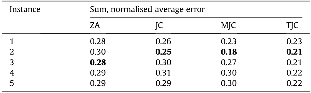
Table 1Results of the optimisation runs for selecting a preferred constitutive model.Five instances of the optimisation were completed for each constitutive model utilising all six experimental conditions.The average error varies from instance to instance for individual strength models due to the probabilistic nature of the optimisation process,in which some iterations identify better solutions than others.

where x is an experimental measurement,x’is the corresponding numerical measurement,i refers to the experiment number,j refers to an individual measurement point in an experiment,and n is the number of measurement points in a specific experiment.

A schematic of the optimisation workflow is given in Fig.9.

The MJC and TJC models are shown in Table 1 to provide the best(lowest error)results,although there is significant variation across the difference optimisation instances.In addition,each optimisation run,for each constitutive model,found a significantly different set of hyperparameters.This suggests that either the BO algorithm was not able to fully converge within its iteration budget,or that the solution is non-unique.This will be further investigated in Section 5.

The best result for each constitutive model option is plotted in Fig.10 for each of the six experiments.We can observe that for the penetration versus time experiments(experiment 1 and 2)there is little differentiating between the four models.Experiment 2 is a better choice for evaluation as there is less scatter in the measurement points.For experiment 2 the JC model is shown to provide the best agreement with the measurements,while the ZA,MJC,and TJC are all comparable.At the final measurement point these models are underestimating penetration by approximately 0.2 mm(4.5%).For the rod-on-anvil experiments(exp.3 and 4)the MJC and TJC models are clearly superior to the ZA and JC models,particularly in the intermediate positions between 2.5 and 10 mm from the nose where the JC and ZA models exhibit bulking that is not measured in the experiments.For the blast experiments,none of the simulations can exactly replicate the shape of the plate measured in the experiments,consistent with the initial publication[22],potentially due to discrepancies between the experimental and numerical setups(e.g.,simulations used C4 explosive while experiments used PE4,simulations modelled a circular plate while experiments used a square plate,etc).Nonetheless the general shape of the deformed plate and the magnitude of the peak deformation are well reproduced.The TJC model is shown to be the least accurate in predicting the peak of the plate bulge,underpredicting by 4.8% and 7.8% in experiments 5 and 6,respectively.The MJC result is shown to match the profile most closely between 0.02 and 0.1 mm,however the peak of the bulge is best predicted by the ZA and JC models.

The difference between the TJC and MJC constitutive models is in their strain rate hardening formulation.The MJC model uses a single power law term,see Eq.(3),while the TJC model includes an additional power law term,enabling two-part rate hardening behaviour to be more accurately described.For materials which do not exhibit significant,high rate hardening there is little benefit to the TJC model over the MJC model.Indeed,the additional hyperparameters of the TJC model(11 hyperparameters vs.9 hyperparameters for the MJC model)makes the optimisation more costly.Thus,for the remainder of the investigation we will use the MJC constitutive model.

5.Parameter optimisation

To identify optimal constants(hyperparameters)for the MJC model which are general across the experimental conditions used in the optimisation,we use leave-one-out(LOO)cross validation.LOO is a common process in machine learning for estimating the performance of a model on data which has not been used for training.It is computationally expensive,as it requires a model be trained and evaluated for each example/condition in the training data,however it provides a high level of confidence in the generalisability of the model.As we have six experiments we perform six iterations of LOO cross validation,each iteration involving optimisation on five of the six experiments,e.g.,one iteration of LOO cross-validation would perform the optimisation on experiments 1 through 5,leaving out experiment 6.For each LOO condition we run 20 instances of Bayesian optimisation(BO)according to the methodology described in Section 4.1,with an objective to minimise the error between the experimental measurements and numerical predictions.Classical LOO cross-validation would then apply each set of the LOO-optimised hyperparameters to the leftout experiment,selecting the best(minimum error)candidate from that result.As we have a limited number of experiments,and as those experiments vary widely in their simulated loading conditions,we have elected to apply the best(minimum error)result from each of the six LOO runs to simulate all six experiments,from which the minimum error result is selected as the best solution.

The results of the LOO cross validation are plotted in Fig.11 as a parallel plot of the optimal MJC model hyperparameters resulting from each of the 120 optimisation runs(6 LOO conditions,each with 20 instances),with the best performing results from each LOO run highlighted in red.For readability,the solutions are also provided in Table 2 together with the error from each experimental condition.The best identified hyperparameters shown in Fig.11 and Table 2 do not exhibit any obvious clustering,suggesting that the solution is non-unique,i.e.,there are a range of hyperparameter combinations that can generate comparable results in LS-DYNA.This is not unexpected as the hyperparameters of the MJC model are not independent-for instance the strain hardening response can be well defined by varying subsets of A,B,n,Q,c,Q,c.All of the best(lowest error)solutions describe near zero strain rate hardening(i.e.,β≈0),however as all the experiments used to derive these parameters were highly dynamic there is a limited range of strain rates over which the model is fit.Conventional characterisation experiments may span as many as seven orders of magnitude(e.g.,10sto 10s).In Ref.[1]the rate hardening behaviour of a Class 1 HHA steel is found to be considerably larger than that identified here.What we observe is that the optimisation,in lieu of capturing the full rate dependency,increases the initial yield strength.The effect,when applied to loading rates representative of those included in the experimental conditions considered,is analogous to a lower quasi-static yield strength with higher strain rate dependency.This also explains the findings in Section 4.1,where the TJC model was unable to provide better results than the MJC model due to minimal strain rate hardening.The thermal softening parameters are also found to vary significantly across the optimisation runs,providing solutions across the entire allowable range from 0.5 to 1.5.Although we expected the thermal softening rate to be important in the rod-on-anvil deformation as well as localisation of the cap in the blast experiments,this is apparently not significant.

The stress-strain curves described by the MJC model with hyperparameters from Table 2 are plotted in Fig.12 for quasi-static(10s)and dynamic loading rates(2000 s)at room temperature(293 K).Although the optimal hyperparameters were shown to vary substantially across the LOO conditions,the stress-strain curves described by the resulting models are reasonably consistent.The curves define an initial yield strength of 1850—2250 MPa,near zero strain rate hardening,and thermal softening overcoming strain hardening effects.For comparison we include baseline curves,utilising JC constants from Ref.[12]and TJC constants from Ref.[14](specifically,the GYS compression parameters with a correction to the strain rate and thermal softening terms).A third model,referred to as baseline ZA uses the Zerilli-Armstrong parameters from Ref.[11]that were optimised to fit the 2.90 cm penetration-time experiment from Ref.[12](experiment 1 in this study).The baseline constitutive model constants are provided in the Appendix.

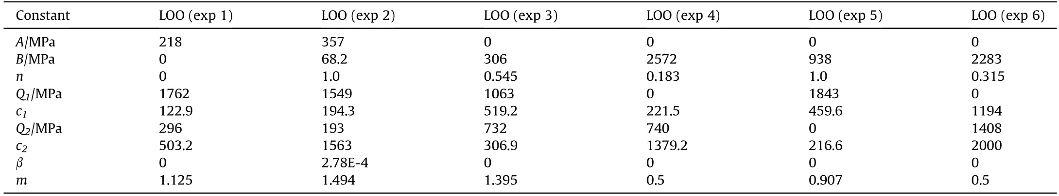
Table 2Optimised modified Johnson-Cook(MJC)model hyperparameters identified using Bayesian optimisation with leave-on-out cross validation(LOO)on six experimental conditions.The experiment noted in the column header is the one“l(fā)eft out”from each LOO iteration.

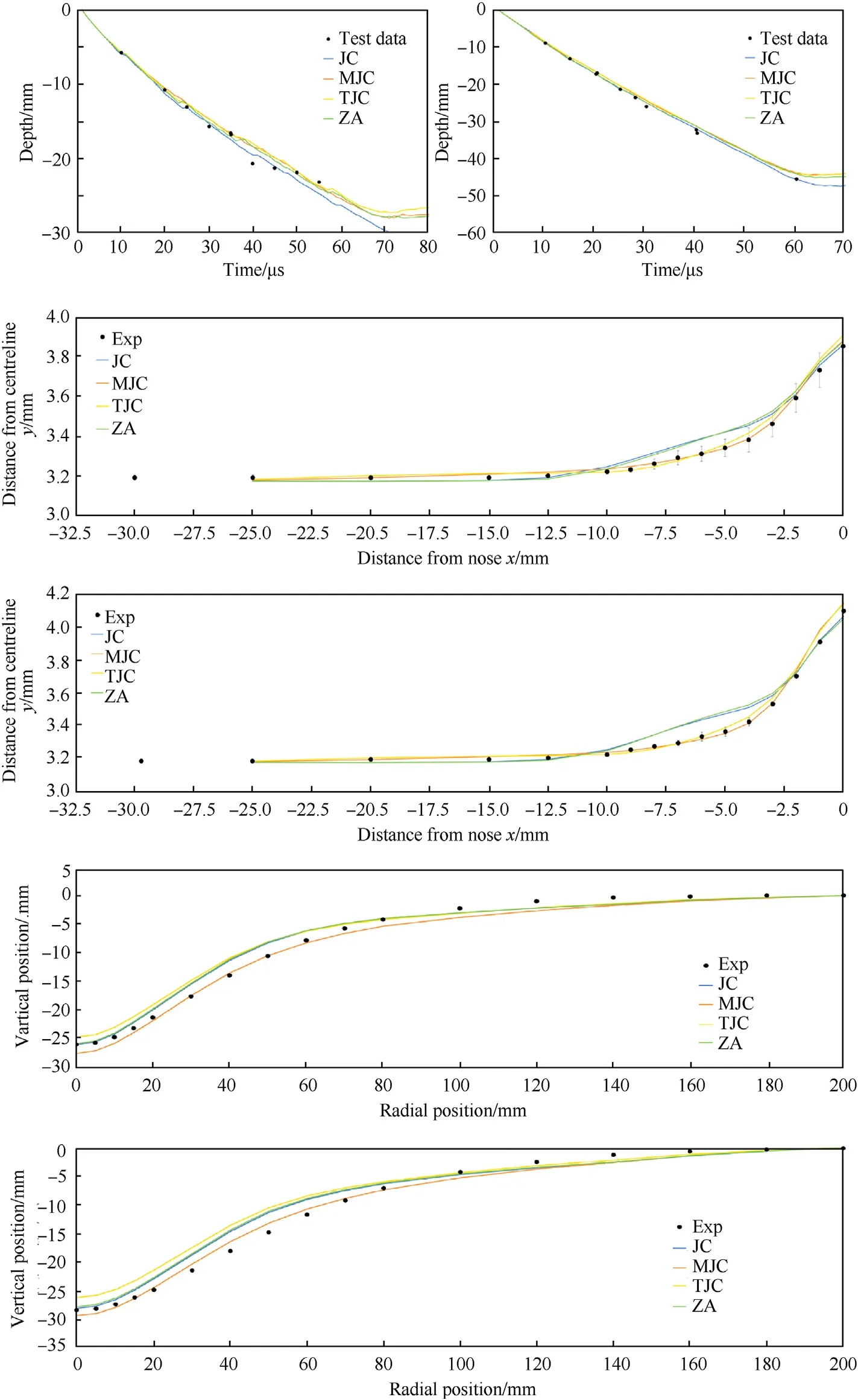
Fig.10.The best numerical result for each of the four constitutive model options plotted together with the experimental measurements.From top-to-bottom:depth of penetration vs time for a WHA rod impacting 2.90 cm thick high-hardness armour steel at 1250 m/s(exp 1,left)and 4.95 cm thick target at 1700 m/s(exp 2,right),final side profile of a highhardness armour steel following impact on a rigid anvil at 184 m/s(exp 3),and at 208 m/s(exp 4),deformed profile of 4 mm thick high-hardness armour steel plates following detonation of a 37.5 g explosive charge at 13 mm standoff(exp 5),and a 57.5 g explosive charge at 25 mm standoff(exp 6).

At quasi-static loading rates the LOO curves are shown to typically describe a harder material than any of the baseline conditions.At dynamic loading rates the TJC model is consistent with the harder curves described by the LOO results,although this indicates that the baseline TJC model has substantially higher rate hardening than any of the LOO solutions.The strain and rate hardening of the baseline JC curve is comparable with some of the LOO results,particularly the LOO exp 3 and exp 5 results.The baseline ZA model is shown to describe a fundamentally different response than the other models.

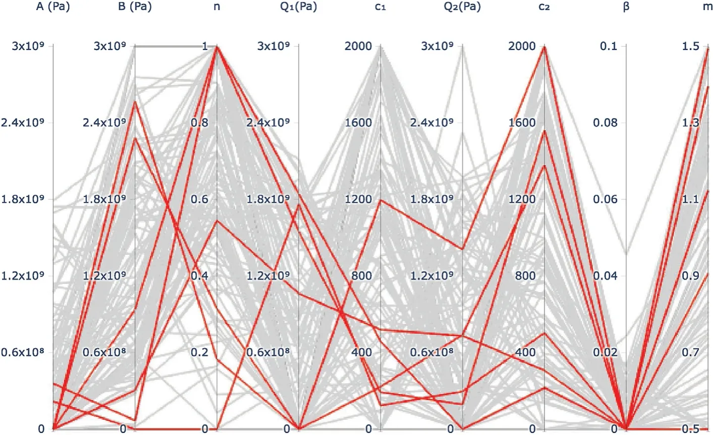
Fig.11.Parallel plot of the MJC model constants/hyperparameters identified in the 120 leave-one-out cross validation experiments.Each x-value represents a constitutive model constant,e.g.A,and the results of each optimisation run are represented by a line series across those variables.The best result for each LOO run is highlighted in red.

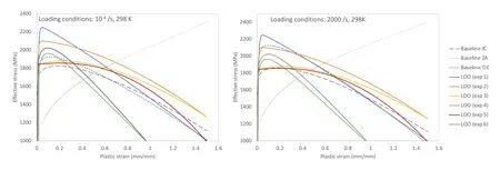
Fig.12.Plasticity curves described by the MJC strength model with optimal hyperparameters identified using Bayesian optimisation with leave-one-out(LOO)cross validation.Baseline curves,representing constitutive models with derived from conventional mechanical characterisation experiments or optimised variants of such,are plotted for comparison.Curves are generated for a strain rate of 10-4 s-1(left)and 2000 s-1(right),at a starting temperature of 298 K.

In Fig.13 we plot the simulation results using the optimal hyperparameters from Table 2 together with the experimental measurements and simulation results generated using the baseline models described previously.For the penetration versus time experiments we see that the LOO results are all relatively similar.In experiment 1,the predicted depth of penetration(DoP)at the final experimental observation varies from 2.25 mm to 2.53 mm(experimental measurement＝2.32 mm).In experiment 2 the predicted depth of penetration at the final experimentalobservation varies from 4.22 mm to 4.55 mm(experimental measurement＝4.56 mm).The LOO(exp 1)and LOO(exp 2)results are shown to slightly under-predict penetration,with the others proving comparable results to the baseline JC and baseline ZA simulations.The TJC results are shown to significantly underpredict penetration for both experiments.As the baseline JC and ZA models were either previously validated against or derived from experiment 1 and experiment 2 measurements,while the baseline TJC model was derived from and validated on a different set of experiments,this result is not surprising.

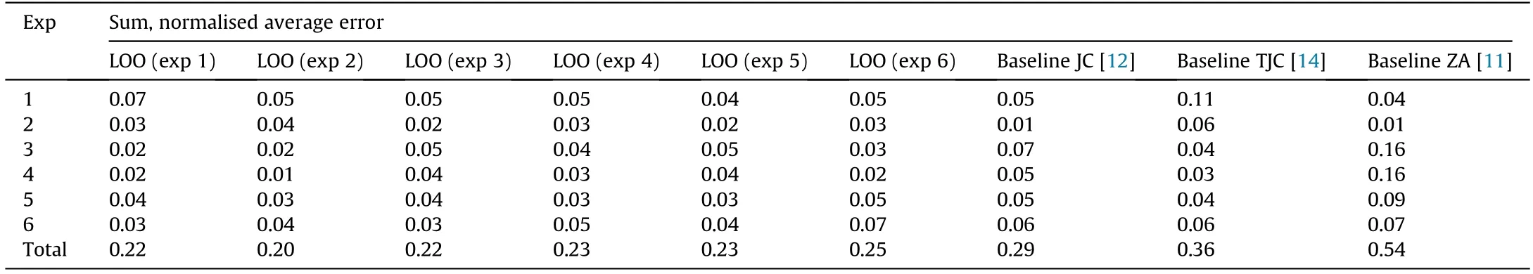
Table 3Total error calculated from the LS-DYNA simulations of the six experiments using the optimised hyperparameters from each leave-on-out(LOO)run compared to baseline results generated from published constitutive model parameters.The sum error is found to be lower for all LOO runs that all three baseline models.

Fig.13.Numerical simulation results generated using the MJC strength model and optimal hyperparameters identified by Bayesian optimisation with leave-on-out cross validation compared with experimental measurements and baseline curves,representing constitutive models with constants derived from conventional mechanical characterisation experiments or optimised variants of such.From top-to-bottom:depth of penetration vs time for a WHA rod impacting 2.90 cm thick(exp 1,left)and 4.95 cm thick(exp 2,right)highhardness armour steel at 1250 m/s and 1700 m/s,respectively;final side profile of a high-hardness armour steel following impact on a rigid anvil at 184 m/s(exp 3),and;208 m/s(exp 4);deformed profile of 4 mm thick high-hardness armour steel plates following detonation of a 37.5 g explosive charge at 13 mm standoff(exp 5),and;a 57.5 g explosive charge at 25 mm standoff(exp 6).

For the rod-on-anvil experiments we see that the LOO results are all reasonably similar,varying at most 0.1 mm on radius along the length of the rod.The baseline JC results are most similar to the LOO(exp 3)and LOO(exp 5)results,consistent with the penetration simulation results and the plasticity curves from Fig.12,while the baseline TJC results show comparable nose deformation to the LOO(exp 1)and LOO(exp 2)results,but with more significant deformation between 2.5 mm and 10.0 mm from the nose.In experiment 3 the radius of the rod nose is predicted to be between 3.86 mm and 3.95 mm,compared with the experimental measurement of 3.85±0.06 mm.In experiment 4 the radius of the rod nose is predicted to be between 4.09 mm and 4.22 mm,comparedwith the experimental measurement of 4.10±0.01 mm.The baseline ZA result is again shown to describe a substantially different response to that observed in the experiment.

For the blast experiments none of the simulation results are unable to exactly match the profile of the experimental plate,consistent with the original publication[17],however the general shape and peak deformation agree very well.The LOO results all describe a reasonably consistent profile,varying by a maximum 5 mm in the vertical position along the span of the plate.The peak deformation is predicted in experiment 5 to be between 2.50 cm and 2.77 cm by the LOO simulations,compared to 2.61±0.01 cm measured in the experiment.In experiment 6 the peak deformation is predicted to be between 2.67 cm and 2.94 cm by the LOO simulations,compared to 2.83±0.01 cm measured in the experiment.The baseline JC and TJC results are extremely similar to the LOO(exp 4)and LOO(exp 6)results,while the baseline ZA model is shown to over-predict the peak deformation for both experiments.

In Table 3 the error for each of the best LOO runs is compared to that of simulations utilising the baseline material models.We observe that all six of the best LOO results provide a lower error than the baseline JC,TJC,and ZA models.Recall that the HzB steel used by Ref.[12]in the penetration vs time experiments is a different material to the HHA steel used by Refs.[14,17]for the rodon-anvil and blast experiments.The nominal properties of those two materials are comparable,however,and thus were included together in the optimisation activity.Based on the results of the optimisation and the plots in Fig.13 we can conclude that the HzB steel appears to perform marginally softer/lower strength than the HHA steel.The LOO results that describe the highest strength material,LOO(exp 1)and LOO(exp 2),under-predict the rod penetration in experiment 1 and 2 against the HzB steel,but show excellent agreement with the rod-on-anvil and blast experiments on the HHA steel.Conversely,the LOO results which describe the lowest strength material,LOO(exp 3),LOO(exp 4)and LOO(exp 5)have better agreement with the experiments on the HzB steel but tend to over-predict deformation in the experiments on the HHA steel(see e.g.,experiment 3,LOO(exp 4)result and experiment 6,LOO(exp 3)result).The variation,however,is marginal,confirming the validity of our earlier assumption that the HzB and HHA steels are similar enough to be adequately modelled with the same material model.

6.Evaluation

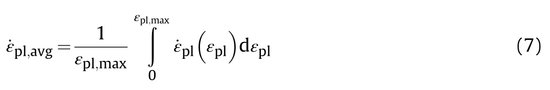
The best LOO result is shown in Table 3 to be found during the LOO(exp 2)run,with a sum average error of 0.20.This is slightly more than the best result from the initial experiments of 0.18,see Table 2.The initial evaluation was optimised on all six experiments while the LOO evaluation was optimised on only five experiments,thus a lower error should be achievable.However,we utilise the LOO cross validation to promote the generalisability of the solution to prevent overfitting.The optimised hyperparameters are hypothesised to be applicable across the range of loading conditions experienced by the material in the six experiments considered.To define this range we interrogate the strain,strain rate,temperature,and stress triaxiality present during simulation of the experiments.For the penetration experiments we track these variables in two columns of target elements through the thickness,(1)along the axis of symmetry and(2)aligned with the outer edge of the projectile.For the rod-on-anvil simulations we track these variables in a row of elements along the length of the rod at the outer surface,and in a radial progression towards the axis of rotation on the nose surface.For the blast simulations we track these variables along a row of elements on the rear surface of the plate covering the entire radial span.The strain,strain rate,temperature,and stress triaxiality are recorded at a high frequency(1.0×10s intervals)and are averaged in terms of plastic strain increment.For example,the average strain rate in each tracked element is calculated as,

Histograms of the average plastic strain,strain rate,temperature,and stress triaxiality generated from this analysis are shown in Fig.14.Assuming the tracked elements define the most important and representative sections of the steel parts,the histograms can provide an indication of the loading conditions for which the derived hyperparameters are valid.We can observe in Fig.14 that the penetration experiments induce the greatest amount of plastic strain,up to 100%,and all simulations exhibit average plastic strains up to 20%(the blast simulations exhibit the lowest plastic strain).All simulations show elements under highly dynamic loading rates,beyond 100,000 sin the penetration experiments,between 10,000—100,000 sfor the rod-on-anvil,and up to 10,000 sfor the blast simulations.None of the simulations exhibit extreme plastic heating.Most of the simulations have maximum average temperatures below 600 K,with some elements in the penetration simulations marginally exceeding this limit.The triaxiality histogram shows that loading is predominantly in compression(negative triaxialities)for the penetration and rod-on-anvil simulations.The blast simulations show a wide distribution of stress states,distributed across compression(negative triaxialities),shear(zero triaxiality),and tension(positive triaxialities).

To evaluate the generalisability of the optimised MJC hyperparameters we consider a new experimental condition-dynamic compression with a split Hopkinson pressure bar(SHPB)apparatus.There are two experimental conditions available for comparison with numerical simulations,corresponding to an average strain rate of approximately 1000 s(from Ref.[14])and an average strain rate of approximately 2500 s(from Ref.[27]).These strainrates are within the range measured during simulation of the deep penetration experiments(exp 1 and exp 2).We expect near uniaxial compression throughout the experiments,corresponding to a stress triaxiality of-1/3,which is also within the range of experiments used for the optimisation,see Fig.14.Thus,the optimised hyperparameters are expected to be applicable to these experiments.

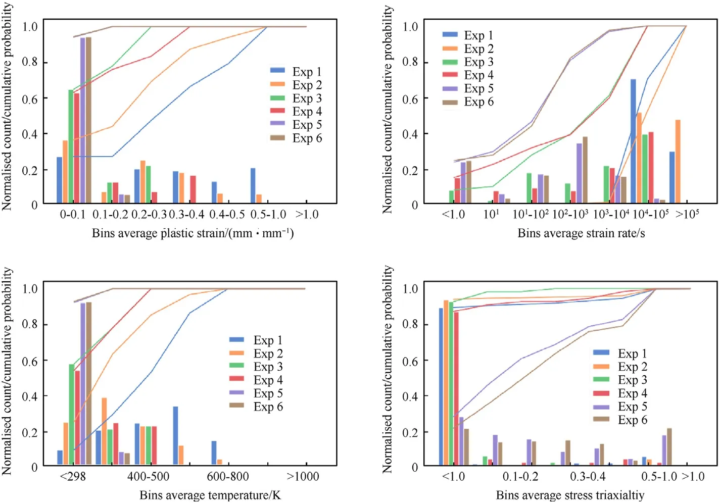
Fig.14.Histograms depicting the average plastic strain(top left),strain rate(top right),temperature(bottom left)and stress triaxiality(bottom right)in selected mesh elements during simulation of the six experimental conditions.The histogram bin counts are plotted as columns and the cumulative probabilities are represented as line plots.

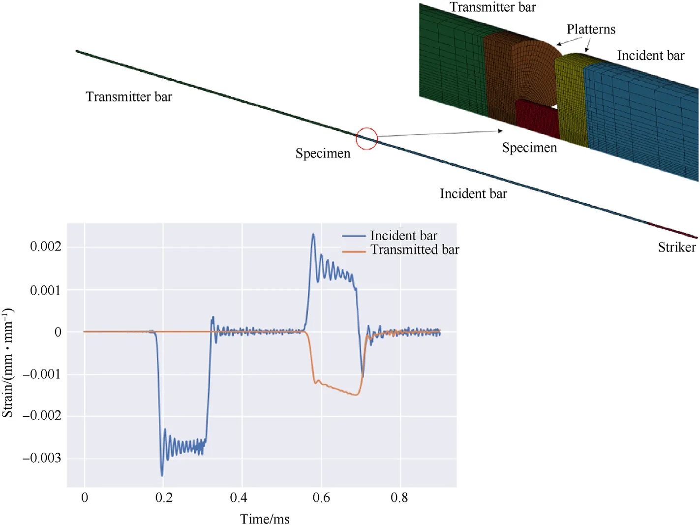
Fig.15.Numerical setup for the compression split Hopkinson pressure bar(SHPB)simulations.The entire SHPB apparatus is modelled,the test specimen is shown in the inset.During the simulations elastic strain is measured on the incident and transmitter bars at locations nominally identical to the experimental equipment.An example of the numerical strain signal in the incident and transmitter bars is provided,from which strain rate,engineering strain and engineering stress are calculated.

For the simulations we model the full SHPB apparatus,measure elastic strains on the incident and transmitter bars in the same location as the experimental gauges and calculate the engineering stress vs.engineering strain response of the specimen.Simulations were performed in LS-DYNA using 3D,quarter symmetry.The full SHPB apparatus and test specimen were modelled using 8-node,reduced-integration(constant stress)hexahedral solid elements forthe steel specimen.The maraging steel incident and transmitter bars as well as the platterns are modelled as elastic materials.The numerical setup is shown in Fig.15 together with an example strain pulse recorded during a simulation.

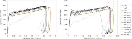
Fig.16.Comparing experimental engineering stress vs strain signals recorded in compression split Hopkinson pressure bar experiments and simulations at approximate strain rates of 1000 s-1(left)and 2500 s-1(right)with numerical predictions.

The simulation results are plotted in Fig.16 for the best LOO solutions from Table 2,the baseline constitutive models introduced in Section 5,and the best MJC result from the initial constitutive model selection activity that provided the minimum total error of all optimisation runs(Instance 2 in Table 2,labelled as“MJC best”in the figure).We can observe that the simulation results using the different LOO hyperparameters vary significantly.However,of note is that the numerical curves showing best agreement with the experimental measurement are those from the baseline TJC,LOO(exp 1),and LOO(exp 2)hyperparameters.These LOO results are those which corresponding to the two minimum error results in Table 3.The“MJC best”curve agreement is comparable with that of the LOO(exp 1)results but inferior to the LOO(exp 2)results,suggesting that those hyperparameters also provide a very good solution across the loading conditions considered.The baseline TJC model is shown to agree extremely well with the SHPB signal,as expected given that it has been derived in part through inverse modelling of these exact experiments.The baseline JC model is found to be comparable to the LOO(exp 3)and LOO(exp 5)results,consistent with previous findings.The baseline ZA model,again,describes material response significantly different to that exhibited by the experimental specimen,further highlighting the risk of optimising constitutive model constants for a single experimental condition.

7.Conclusions

We have developed a Bayesian optimisation methodology to derive viscoplasticity model constants from functional experiments,i.e.,those which serve an additional function beyond just that of identifying constitutive model constants.The methodology has been applied on high hardness armour steels,where we attempt to minimise the error between numerical simulation predictions and experimental measurements of(1)time-resolved penetration of long rod projectiles,(2)near-field explosion bulging,and(3)rodon-anvil deformation.To maximise the general applicability of the optimised solution we employ leave-one-out cross validation,a typical strategy in machine learning used to minimise the likelihood of overfitting.The generalisability of the optimised solution was demonstrated via numerical simulation of an experimental condition not considered in the optimisation,namely dynamic compression in a split-Hopkinson pressure bar.The simulations demonstrated excellent agreement with the measured result.The numerical simulations utilising constitutive model parameters derived with our Bayesian optimisation methodology were demonstrated to provide superior agreement with experimental measurements than simulations which utilised conventionally derived parameters and those optimised on a single experimental condition.

The presented methodology is expected to be generally applicable,i.e.,optimal model constants can be derived for any material whose performance is well described by a constitutive model,provided that adequate experimental measurements are available.The applicability of such derived parameters is defined by the range of experimental conditions used during the optimisation,i.e.,experiments which span a broader range of loading conditions will provide a more widely applicable material model.

The authors declare that they have no known competing financial interests or personal relationships that could have appeared to influence the work reported in this paper.

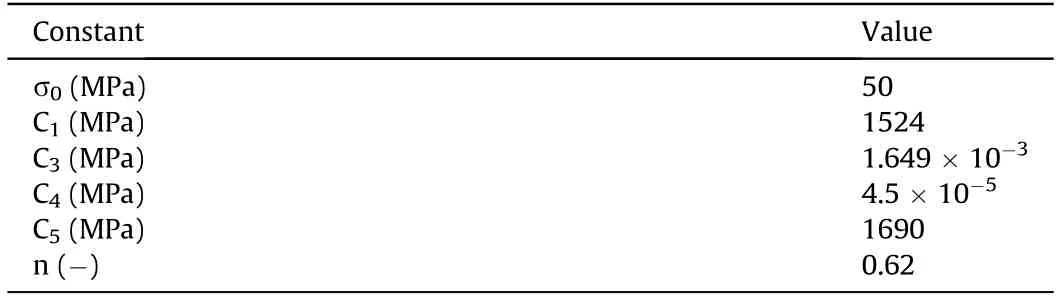
Table A1Constitutive model parameters of the baseline ZA model from Ref.[11].

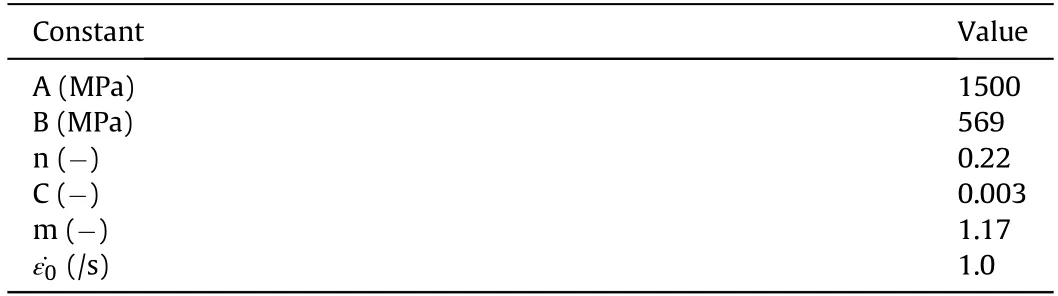
Table A2Constitutive model parameters of the baseline JC model from Ref.[12].

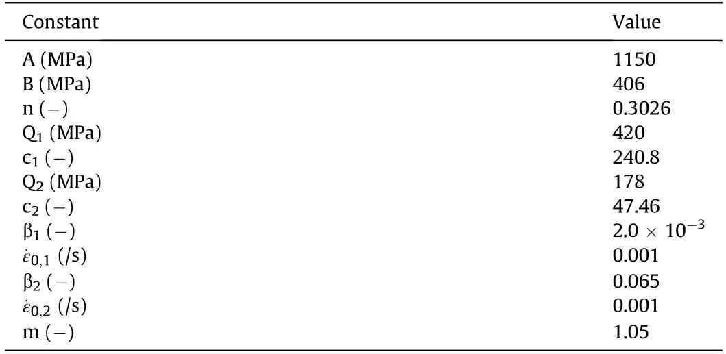
Table A3Constitutive model parameters of the baseline TJC model from Ref.[14].