
Ballistic response of armour plates using Generative Adversarial Networks
2022-09-22 10:49:36ThompsonTeixeirDisPulinoHmilton
Defence Technology 2022年9期
S.Thompson ,F.Teixeir-Dis ,*,M.Pulino ,A.Hmilton
a Institute for Infrastructure and Environment(IIE),School of Engineering,The University of Edinburgh Alexander Graham Bell Building,The King's Buildings,Edinburgh,EH9 3FG,United Kingdom
b School of Engineering,Faculty of Science,Engineering and Built Environment,Deakin University Waurn Ponds,Victoria,3220,Australia
c Data Science and AI,Engineering,Group Chief Information O Ce,Lloyds Banking Group,69 Morrison St,Edinburgh,EH3 8BW,United Kingdom
Keywords:Machine learning Generative Adversarial Networks GAN Terminal ballistics Armour systems
ABSTRACT It is important to understand how ballistic materials respond to impact from projectiles such that informed decisions can be made in the design process of protective armour systems.Ballistic testing is a standards-based process where materials are tested to determine whether they meet protection,safety and performance criteria.For the V50 ballistic test,projectiles are fired at different velocities to determine a key design parameter known as the ballistic limit velocity(BLV),the velocity above which projectiles perforate the target.These tests,however,are destructive by nature and as such there can be considerable associated costs,especially when studying complex armour materials and systems.This study proposes a unique solution to the problem using a recent class of machine learning system known as the Generative Adversarial Network(GAN).The GAN can be used to generate new ballistic samples as opposed to performing additional destructive experiments.A GAN network architecture is tested and trained on three different ballistic data sets,and their performance is compared.The trained networks were able to successfully produce ballistic curves with an overall RMSE of between 10 and 20 % and predicted the V50 BLV in each case with an error of less than 5 %.The results demonstrate that it is possible to train generative networks on a limited number of ballistic samples and use the trained network to generate many new samples representative of the data that it was trained on.The paper spotlights the benefits that generative networks can bring to ballistic applications and provides an alternative to expensive testing during the early stages of the design process.
1.Introduction
Predicting the outcome of impulsive events such as ballistic impacts is a complex problem for researchers due to the difficulties in characterising material behaviour across a wide range of loading rates and impact scenarios.In terms of analysis,it is the combined sum and influence of a number of input variables that ultimately govern the response of a material and structure under a specific impulsive loading scenario.Approaches to understand such events include highly empirical(i.e.experimental[1,2])and semianalytical and numerical methods that are designed to mimic experiments[3].However,using these methods to make predictions outside the range of responses of the empirical data set from which the analysis has been derived often leads to inaccurate results[4].
Machine learning techniques are well suited to classification and regression problems,particularly those in high dimension problem spaces such as dynamic impact events where there are many influential parameters that govern the response of the structure.In that sense,machine learning can allow impact events to be characterised and predictions can be made without the conventional limitation on the number of input variables or dimensionality of the problem.Problems with a larger dimensionality,however,require more comprehensive training data and thus the range of application for the machine learning algorithm is defined by the limits of the training data set[4].A good dataset used to train machine learning models should be of both sufficient size and sufficient quality,where size refers to the total number of samples and quality refers to the reliability(i.e.the degree to which the datacan be trusted)and feature representation(i.e.the degree to which the data includes the features of interest in the problem space)in the data set.Machine learning is an application of Artificial Intelligence(AI)that provides systems with the ability to improve and learn from experience without the explicit need for programming.The term“artificial intelligence”was first coined by McCarthy in 1956[5]in the first academic conference on the subject.Since then researchers have made much progress widening the influence that machine learning techniques have in the world.Home voice assistants and self driving cars are becoming common and are made possible by Artificial Neural Networks(ANN)that have been modeled loosely after the human brain.Neural networks are essentially a set of algorithms that are designed to recognise numerical patterns contained in vectors,into which real-world data such as images,text or time series must be translated.The basic building block of the ANN is the perceptron(or node)which exists as a linear classifier—it produces a single output based on several inputs by forming a linear combination of the input and the respective weight that it has assigned to the input to determine its significance.Nodes can be arranged in many different ways to form different neural networks to suit the task in hand and the type of data it will be working with.For example,Long Short-Term Memory(LSTM)networks are a class of ANN where connections between nodes form a directed graph along a temporal sequence—the impact of which has been notable in language modelling and speech-to-text transcription and are crucial part of what makes voice home assistants function[6].A Multi Layer Perceptron(MLP)is a deep artificial neural network composed of more than one perceptron.It is composed of an input layer to receive the signal,an output layer that makes a decision or prediction regarding the input and the hidden layers that are the computational engine of the MLP.These networks are often applied to supervised learning problems where they train on a set of input-output pairs and learn to model the correlation(or dependencies)between those inputs and outputs.Training involves adjusting the parameters of the network such that the error is minimised.Once a model is trained,it is possible to provide it with new inputs and predict new outputs as a function of what the model has learned.
A schematic of a projectile perforating an armour plate is shown in Fig.1.In a previous publication by the same authors,two MLP networks were used to predict the residual velocity(v)of blunt projectiles perforating multilayer metallic armour systems[7]:(i)one was trained on a data set generated by a validated analytical model and(ii)another one trained solely on experimental data.The model was trained to understand the ballistic response of the metallic plates and predict the residual velocity for a given impact velocity,layer thickness and set of material properties.The model proved successful in making predictions on monolithic cases with an error of less than 10 %.However,the statistical quality of the experimental data set used to train the MLP network suffered from a high degree of clustering about impact conditions and material choice.This is expected to be the case in any terminal ballistics problem where the cost of testing will naturally limit its scope[4].
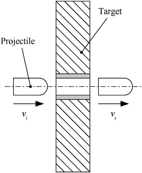
Fig.1.Projectile perforating an armour plate:vi is the impact velocity and vr is the residual velocity.
2.Generative Adversarial Networks
The Generative Adversarial Network is a framework that was first proposed by Goodfellow et al.[8]for estimating generative models via an adversarial process,in which two neural networks compete against one another and are trained together.It is a machine learning technique that learns to generate fake samples indistinguishable from real ones via a competitive game.
For a machine learning application,a perfect training set should include observations from experiments performed across a range of impact velocities with different materials and different armour system configurations(i.e.different thicknesses).However,due to the destructive nature of these tests,there is a high cost associated with ballistic experiments.As a potential solution to this problem,this paper proposes the use of a different neural network,a GAN,that has been specifically developed to supplement ballistic data sets.A Generative Adversarial Network is a more recent class of machine learning system that has the ability to generate entirely new data and make predictions through unsupervised learning[9].Given a training set,this technique learns to generate entirely new data with the same statistical representation as the training set.This allows additional ballistic samples to be generated using the model as opposed to performing additional destructive tests.
The base architecture of a GAN is composed of two neural networks:a discriminator and a generator,as shown in Fig.2.The discriminator D is set up to maximise the probability of assigning the correct labels to real and fake samples.Meanwhile,the generator G is trained to fool the discriminator with synthesised data[10].In other words,D and G play the following two-player minimax game with value function V(G,D)[8].

where x is the input to D from the training set,z is a vector of latent values input to G,Eis the expected value over all real data instances,D(x)is the discriminator's estimate of the probability that real data instance x is real,Eis the expected value over all random inputs to the generator and D(G(z))is the discriminator's estimate of the probability that a fake instance is real.The primary goal of G is to fool D and produce samples that D believes come from the training set.The primary goal of D is to assign a label of 0 to generated samples,indicating a fake,and a label of 1 to true samples,that is,samples that came from the training set.The training procedure for G is to maximise the probability of D making a mistake,i.e.an incorrect classification.In the space of arbitrary functions G and D,a unique solution exists,with G able to reproduce data with the same distribution as the training set and the output from D≈0.5 for all samples,ultimately indicating that the discriminator can no longer differentiate between the training data and data generated by G.
2.1.Training sets
The primary goal of this work is to develop a new GAN architecture capable of generating new predictions representative of those originated in ballistic impact experiments.Ballistic testing is a standards-based process where materials are tested todetermined whether they meet protection,safety and performance criteria.In this paper,ballistic experiments refer to the Vballistic test,where projectiles are fired at higher velocities to determine a key design parameter known as the Ballistic Limit Velocity(BLV).In this scope,the BLV is the minimum projectile velocity that ensures perforation[11,12].This velocity is a property of the threatarmour system and is determined by a number of parameters,such as the projectile and target material properties,projectile mass and target configuration(e.g.thickness).This work aims to reduce the costs associated with ballistic experiments by minimising the number of experiments performed and supplementing the data set by using the GAN model instead.It discusses and compares the results from three separate GAN models trained on three separate training sets.An appropriate training set is required such that the discriminator can learn the distribution of the data.
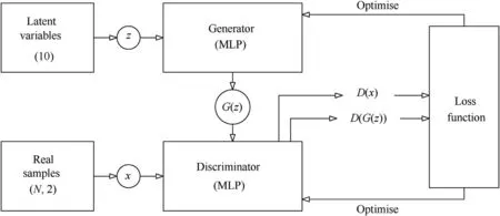
Fig.2.Schematic diagram of a Generative Adversarial Network(GAN).
In this case,the generative networks are trained to generate new samples of ballistic data.It is therefore important to prepare an appropriate data set that can be used for this purpose.
The post-impact residual velocity can be calculated with the relation proposed by Lambert and Jonas[13]:
where v,vand vare the impact,residual and ballistic limit velocities(BLV)for an orthogonal impact,respectively,and a and p are coefficients that govern the shape of the ballistic limit curve.The effect of these parameters on the shape of the curve is shown in Fig.5.The residual velocity is the projectile velocity after it has perforated the target.The definition of the BLV implies that if v=vthen v=0,that is,the residual velocity is zero if the target is struck by a projectile at its BLV[14].In this work,Eq.(2)was initially used to generate ballistic data.
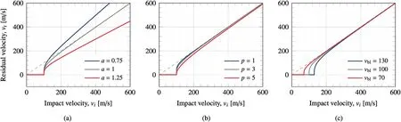
Fig.5.The effect that modifying the Lambert parameters has on the shape of its ballistic curve.Default Lambert parameters used are a=1,p=3 and vbl=100,plot(a)shows the effect of changing parameter a,plot(b)shows the effect of varying parameter p and(c)the variation of vbl.
In order to test the capabilities of this method,the samples generated by the GAN are compared with the equivalent values produced by the Lambert and Jonas relation(Eq.(2)).This was selected for two reasons:(i)the Lambert and Jonas equation can be used to generate the training sets for each test case to effectively test proof of concept,and(ii)it provides a useful metric through which to directly compare the results of the GAN predictions.
Three different test cases were considered,leading to three different training sets to test the performance of the proposed GAN architecture.Each training set is a(N,2)array where N is the number of samples in the training set,the first column corresponds to the impact velocity vand the second column to the residual velocity v.Case 1 represents a best case scenario and consists of 100 logarithmically spaced data points to maximise the number of points around v.These points represent vwith the corresponding vcalculated using Eq(2)and the parameters listed in Table 1.The Case 1 training set,shown in Fig.3(a),covers a wide range of impact velocities,including impacts for velocities both above and below the BLV,providing the learning algorithm with the best chance to learn an idealised representation of the data.Case 2,shown in Fig.3(b),consists of 50 randomly generated data points in the residual velocity test range,which in this case is[0,600]m/s.The training set used for Case 2 is therefore less structured and less dense than Case 1.The final test case is the most realistic and attempts to replicate experimental data in the form that is typically found published in the literature[15—21].10 points were generated at random in the residual velocity test range[0,600]m/s and similarly arranged into a[10,2]matrix.A±10%artificial noise was added to vto mimic experimental measurement error,ensuring that the training data no longer sits on the Lambert ballistic curve,as can be seen in Fig.3(c).
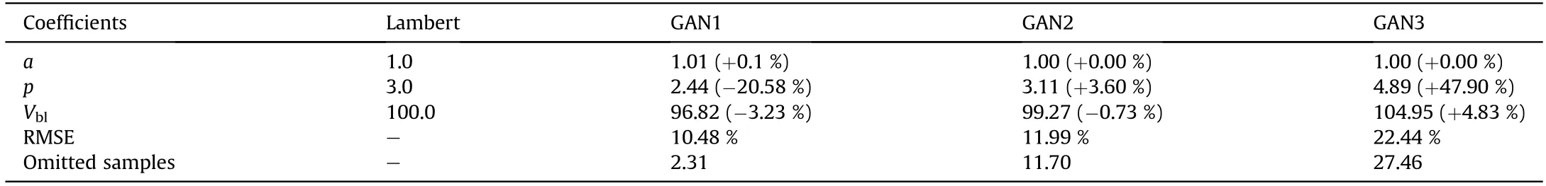
Table 1Lambert parameters used to create the training sets and test each GAN model.
Each of the training sets were normalised between the range[0,1]before training commenced.It should be noted that the numeric values in the dataset are transformed via a common scale,without distorting differences in the ranges of values or losing any information.After training,the output from G is scaled back to original values by using the same object to undo the transformation.For each test case,the trained GAN model generates 100 samples and the curve is fitted in accordance with the Lambert and Jonas model with respect to parameters a,p and vto obtain a new set of Lambert parameters specific to the GAN-generated data and curve.Due to the stochastic nature of generative models,this is performed 100 times for each test case and the average values for each parameter are recorded and compared.
2.2.Model architecture
Multi-Layer Perceptron(MLP)networks were used to create theG and D networks as MLPs are well equipped to deal with regression tasks and the adversarial modelling framework is straight forward to apply when both models are MLPs[8].An MLP network consists of at least three layers of nodes:an input layer,a hidden layer and an output layer.Each layer within an MLP network exists as an arrangement of nodes(perceptrons)and can be visualised as a place where computation occurs.Each node combines data from the input with a set of coefficients,or weights,that either amplify or dampen that input and thereby assign significance to inputs with regard to the task that the algorithm is trying to learn.These inputweight products are summed and passed through the nodes’activation function to determine whether,and to what extent,the signal should progress through the network and influence its final output.A node within an MLP network performs a function that takes in multiple inputs and produces a single output.This function is made up of two parts:(i)a weighted sum of all the inputs plus a constant(bias),and(ii)an activation function.The operation at a node can be described mathematically as:
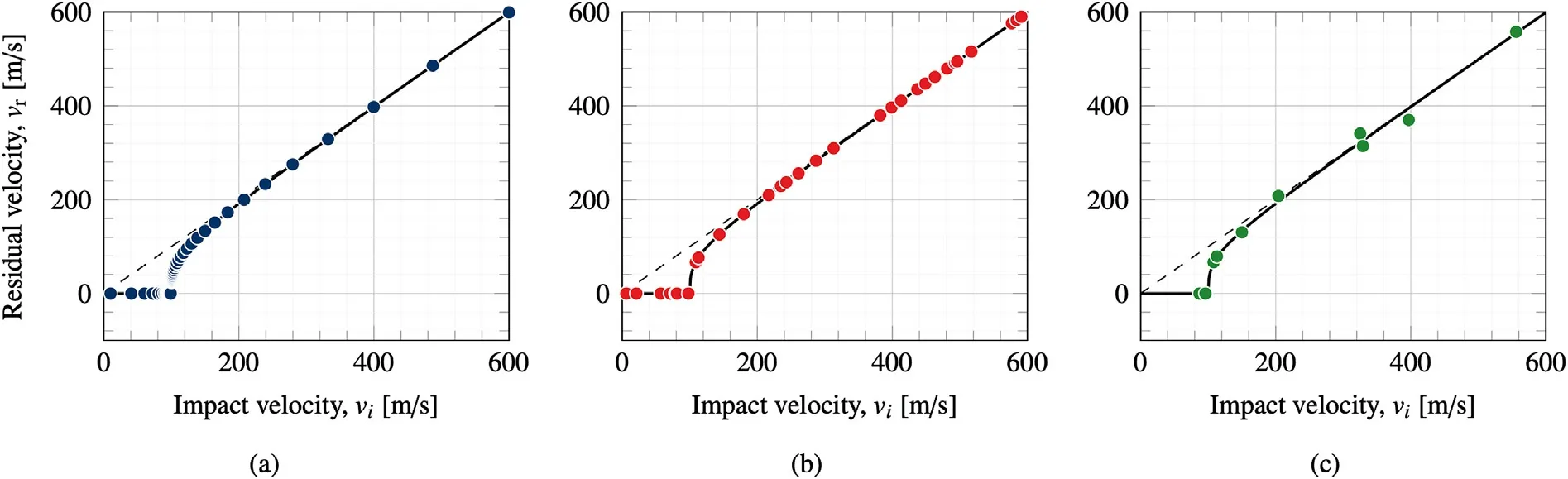
Fig.3.Training sets used to train each GAN model:(a)Case 1,(b)Case 2,and(c)Case 3.
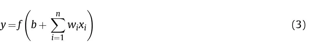
where y is the output,wis the vector of weights,xis the vector of inputs,b is the bias constant and f is the activation function.Adjusting the weights and bias at the node makes it possible to change y to more closely match the desired output,hence training the network.Fig.4 shows a schematic of the operations that occur at a single node within a neural network.More complex operations can be performed when these nodes are combined and arranged into layers to create a mesh-like network.The term deep learning is given to networks composed of multiple hidden layers.
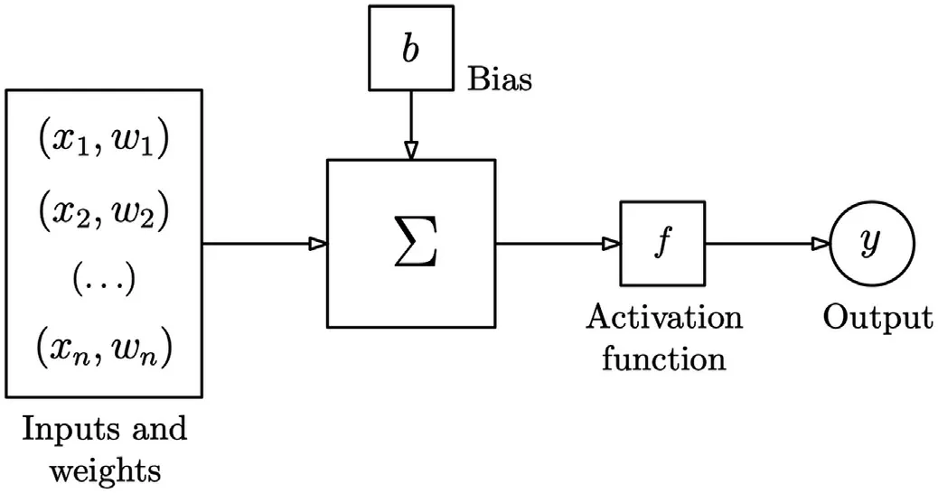
Fig.4.Schematic representation of an active node in an MLP neural network(adapted from Teixeira-Dias et al.[7].
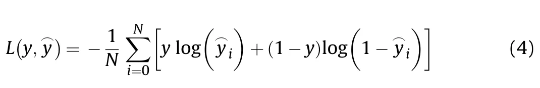
The discriminator takes an instance from either the generator or training set as input,and outputs a classification prediction as to whether the sample is real or fake.It is a binary classification problem.The discriminator network is an MLP network with 5 fully connected(FC)hidden layers,with 25,15,15,5 and 1 nodes in each layer.The model minimises the following binary cross entropy loss function:

The generator model G takes an input z from the latent space and generates a new sample.A latent variable is a hidden or unobserved variable,and the latent space is a multi-dimensional vector space of these variables.Model G uses 10 latent variables as input to the model that exists as a 10 element vector of Gaussian random numbers.The majority of GANs published in the literature focus on using GANs for image generation and analysis.The intentions of the model proposed in this paper differ from the literature in the sense that the training sets used to train the models are smaller and contain fewer data,and secondly the desired output is less complex(training sets considered consist of 100,50 and 10 samples with two features as opposed to commonly used MNIST[26]and CIFAR10[27]image datasets that contain 60,000 and 10,000 image samples respectively with 28/32 features depending on the size of the image).As a result,the authors considered a smaller range of latent input sizes between 2 and 30 and found that a latent input of 10 resulted in a stable model that was able to capture the key features of ballistic curves consistently for different datasets.G has two fully connected hidden layers with 11 hidden nodes and is activated with a Rectified Linear Unit(ReLU)activation function.The weights associated with each node are initialisedwith uniform scaling between 1 and 10.The output layer has two nodes for the two desired elements vand v,and a linear activation function is used to output real values.The network architectures for both models are listed in Table 2.
2.3.Training algorithm
The machine learning algorithm was written in Python 3,using TensorFlow's high-level Keras API for building and training deep learning models.The training process takes place over 1 million iterations and a single iteration is completed once the machine learning algorithm has completed an entire pass through the training data set(one epoch).Within each iteration,the trainable parameters of both the D and G networks are updated alternatively;first the D network is trained and then the G network.D is simply a classifier that learns to distinguish real data(label=1)from fake data generated by G(label=0).It treats data labelled 1 as positive examples during training and data labelled 0 as negative examples,and updates parameters accordingly via the binary cross entropy loss function and adam optimiser.D can therefore be trained alone and is trained on both data from the training set and also from fake data generated by G.The D network is therefore trained on two epochs of data per iteration and,if left uncorrected,would train at a faster rate than G,thus giving D an advantage and therefore affecting the competitive nature of the adversarial process.In order to correct this,the entire sample fed to D is split in half to form a batch.This is done randomly at each iteration to ensure that the total data that D is trained on per iteration is the same as that of G.The G network is trained entirely on the performance D and its trainable parameters are optimised in accordance with its output D(G(z)).
A single iteration of training is complete once the trainable parameters of both the D and G networks have been updated,twicefor D(on real and fake samples)and once for G.First,real samples from the training set X are prepared and passed into D to obtain D(X).A target label of 1 is concatenated with the training data to identify them as real samples.The output D(X),i.e.its prediction as to whether the sample is real or fake,then passes into the loss function and the trainable parameters of D are optimised with the intention of returning a value closer to the target label of 1 for the next real sample it receives.Similarly,D is also trained on fake data from G in the form of G(z)and is concatenated with a target label of 0 to identify them as fake samples.D(G(z))then passes through the loss function and the trainable parameters of the D network are updated with the intention of D(G(z))returning a value closer to the target label 0 for future fake samples.The goal of G however,is to generate samples that D believes to have come from the original training set X,therefore the output D(G(z))is used to train the G network.This defines the zero-sum adversarial relationship between the two models.As the training of G depends on D,the network cannot be trained in isolation.A combined model is therefore required to form the GAN.The GAN is a sequential model that stacks both the G and D networks such that G receives the latent Gaussian vector z as input and can directly feed its output into D.To that end,G(z)is concatenated with a target label of 1(indicating a real sample)and the output D(G(z))passes through the loss function and the trainable parameters of G are updated with the intention of D(G(z))returning a value closer to the target label of 1.It should be noted that the binary cross entropy loss function and adam optimiser are also used to train the combined GAN model and that whilst G is being trained,the nodes within each layer of the D network are frozen and cannot be updated;this prevents D from being over-trained on fake examples.The complete training algorithm of the GAN is shown in Table 3.
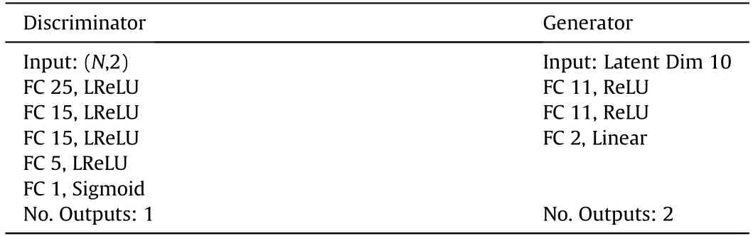
Table 2Architecture of the G and D networks.N is the number of entries in the respective training set.FC refers to a fully connected layer,FC 25 to a fully connected layer with 25 nodes,and LReLU to a Leaky ReLU activation function.
2.4.Model evaluation
This section details the process adopted to evaluate the success of the proposed models.A total of three separate GAN networks have been trained and named in reference to the training set that they were trained on(e.g.GAN1 refers to the generative network trained on the first training set).In this study,the expected values are known as the model is aiming to recreate results representative of the Lambert model.Each model was trained for a total of 1 million iterations and the performance of the GAN was evaluated at every 1000 iterations as the model in its current form was used to generate 100 samples.The RMSE was calculated by taking each vpredicted by the GAN model and computing the difference with the expected value from the Lambert model for the respective v.The non-linear least squares method was used at each evaluation pointto fit the Lambert equation to the generated data such that Lambert parameters specific to the generated model at that point during training could be obtained.The percentage difference of these parameters with the expected parameters,listed in Table 1,was computed and plotted to show how the accuracy of the samples generated by the GAN changes throughout training.This results in four parameters,a,p,vand the RMSE,that are being monitored during training to evaluate the performance of the model.It should be noted that for the model's intended application this would not be the case and instead the generative network would simply be presented with experimental samples that would form the training set.It would have no true reference and as such it can be difficult to know the optimal point in time to terminate the training.
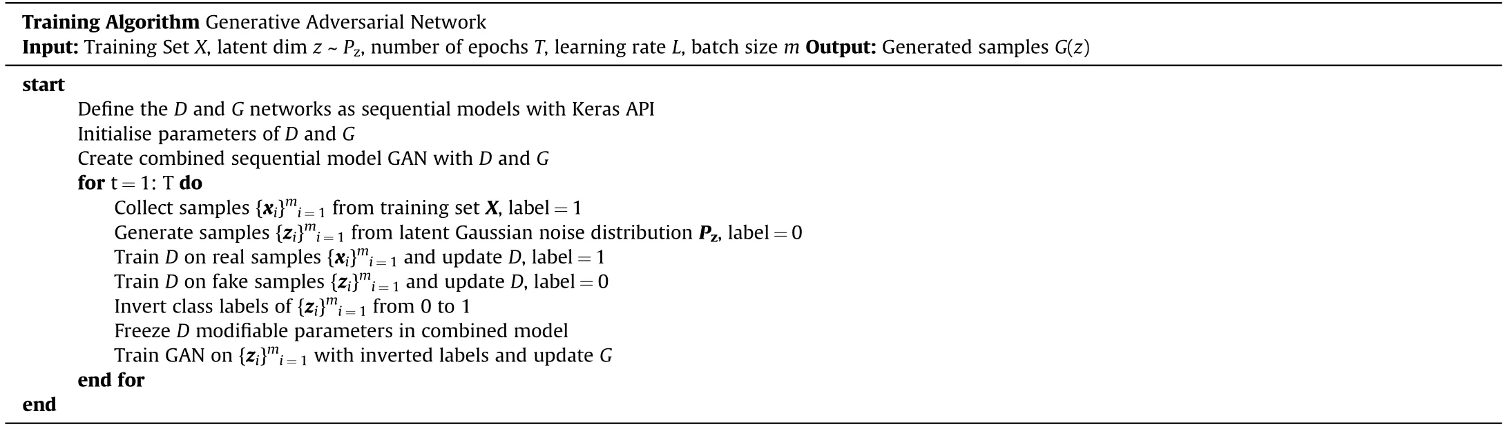
Table 3Training algorithm for the Generative Adversarial Network.
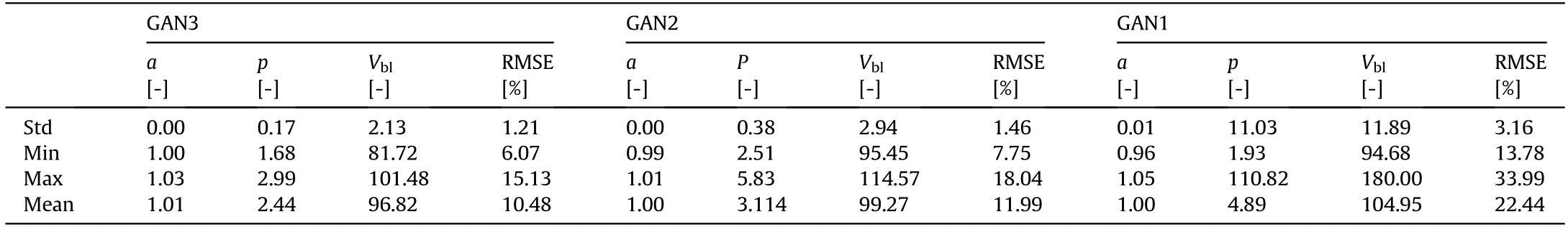
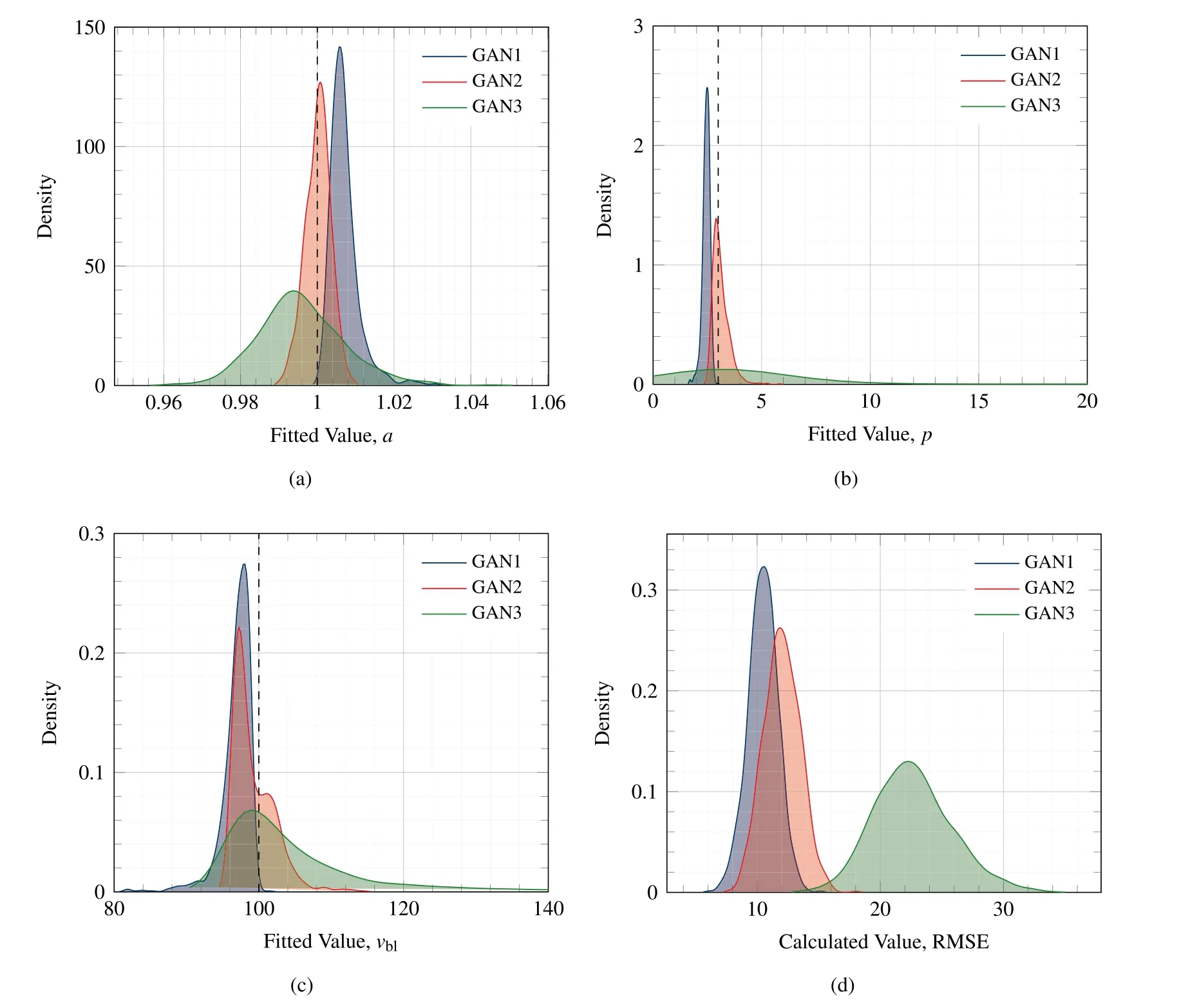
GANs can be very difficult to train and a lot of research is ongoing to improve the convergence of generative networks[28—30].Often the most meaningful way to interpret the success of the GAN is with visual interpretation.It would therefore be recommended to regularly use the GAN during training to generate ballistic samples as an additional qualitative measure to evaluate the training process.That being said,the authors found that for this application 1 million iterations afforded the learning algorithm enough opportunity to consistently optimise the parameters of the network on different training sets,without an unreasonable compromise in computational cost.Once the generative network is trained,it is important to study the quality of the output to determine the success of the model.However,due to the stochastic nature of the GAN and the latent Gaussian input to the network,the output varies.The authors performed a statistical analysis for each of the generative networks to gain further insight into its output.For each of the GAN networks,the 1,000,000th iteration of the model was used to generate 100 samples of data and parameters a,p,vand the RMSE were once again calculated.This was done 1000 times and each of the four parameters were stored at each iteration in a[4×1000]array,the results of which are discussed in the next section.
3.Results and discussion
In this study a total of three separate GAN networks have been trained.The variation of parameters a,p,vand the RMSE are plotted against training time in iterations alongside a 100 sample output of the final model in Fig.6.This is done for each of the three networks,with Fig.6(a)and(b)referring to GAN1,Fig.6(c)and(d)to GAN2 and finally Fig.6(e)and(f)to GAN3.On inspection,it can be seen that the samples generated by each of the GAN networks match the shape of the Lambert curve.In the case of GAN1,which was trained on the first training set,Fig.6(a),there is noticeable improvement in the accuracy of the network as training progresses.Both the RMSE and the respective Lambert parameter errors determined via the fitting model decrease with training.This is a clear indication that the model has learned from the training set and is now able to generate new samples that are representative of that initial data set.This observation is enforced when looking at the samples generated by GAN1 in Fig.6(b).The generated samples appear to come from the same distribution as the training set and display close matching both before and after the ballistic limit.
The training set used to train GAN1 was the most structured and comprehensive of the three training sets and thus provide optimal conditions for the learning algorithm to optimise its respective trainable parameters.Fig.6(c)and(d)show the equivalent results for GAN2.Once again it can be seen that over time the errors of each of the Lambert parameters decrease with training time as the model learns and the output of GAN2 begins to stabilise.Earlier in the training process large error spikes are visible where the output from the model is highly inaccurate.These correspond to points where optimisation was unsuccessful,the loss function would therefore return larger values and the trainable parameters of the network would then be updated more rigorously in order to reduce the loss and improve accuracy.The final iteration of GAN2 was used to generate the 100 samples shown in Fig.6(d).The generated samples are also consistent with those of the Lambert model and representative of the training set that it was trained on.Samples generated by GAN2 demonstrate good matching with the Lambert model past the ballistic limit velocity.However,unlike GAN1,GAN2 does not generate samples below the ballistic limit.The training set used to train the GAN1 model represents an optimal training set and consists of 100 samples logarithmically spaced around the ballistic limit velocity.This provides the GAN model with training data from the entire impact range between[0,600]m/s and subsequently the best opportunity to learn the behaviour of the correct ballistic response.The training set used to train GAN2 however,consists of 50 samples with x values randomly selected between the impact range of[0,600]m/s and the corresponding y values calculated via the Lambert equation.In comparison to the first training set,this data is unstructured and no priority has been made to organise the data around the ballistic limit.Of the 50 samples in the training set,only 7 exist below the ballistic limit.During training,it is likely that GAN2 was optimised such that it converged to a local minima where a solution was found where D believes that samples generated by G belong to the training set-but without including the additional feature that represents the horizontal line at v=0 for v Fig.6.Plots(a),(c)and(e)show the error of the model during training including the RMSE and the percentage difference of fitted Lambert parameters with that used in the original Lambert model.Where a%refers to the percentage error of the fitted parameter specific to the GAN network at that point in training with the true Lambert value a etc.Plots(b),(d)and(f)show a 100 sample output of the networks GAN1,GAN2 and GAN3 after 1 million iterations respectively,where the respective D and G models were trained with a Learning Rate(LR)of 0.0035.Plot includes omitted values that meet either of the elimination criteria:(i)if vi The results of GAN3 are shown in Fig.6(e)and(f).GAN3 was trained on the training set that was the least comprehensive and most representative of data collected via experiments.This training set contains much fewer samples and,unlike training sets 1 and 2,was tainted with additional noise of up to 10 %,to mimic experimental measurement errors.Fig.6(e)shows the variation of parameter accuracy during training.This time the model did not converge as successfully as with GAN1 and GAN2,and appears to be less stable demonstrating more spikes in error throughout training.This being said,Fig.6(f)shows the 100 samples from the final iteration of GAN3 and it can be seen that once again the samples follow the shape of the ballistic curve.The samples generated by GAN3 have a larger spread than those generated by GAN1 and GAN2,but this is consistent with the tainted training set that it was trained on.GAN3 does not demonstrate samples for impact velocities vbetween the range[0,v],however this is expected as samples within that range are not present in the training set.A comparison of the coefficients generated by the final iteration of each GAN network can be found in Table 4. The results in Table 4 compare the average Lambert coefficients determined by curve fitting the samples generated by each of the GAN networks 1000 times with the baseline Lambert parameters defined in Table 1.The results show that all of the GAN networks performed well with respect to parameter a with the percentage error in each case<0.1%.GAN2 was the most successful in regards to p with an average error of 3.6%,outperforming GAN1 and GAN3 which had errors of-20.58 % and 47.90 %,respectively.This remains true for the vcase as GAN2 also produced the lowest average errors of-0.73 %,GAN1 predicted the vwith an error of 3.23 % and finally GAN3 with an error of 4.83 %.This metric is particularly useful as the vis an important parameter when determining the ballistic response of materials and for all GAN networks the predictive error was<5%.Fig.5 shows the influence that parameters a,p and vhave on the ballistic curve.In each case,the Lambert plot with the default parameters listed in Table 1 is shown and Fig.5(a),(b)and(c)show how the plot changes by varying a,p and v,respectively. Fig.5(a)demonstrates that decreasing a raises the profile of the curve and increasing it does the opposite.a=1 assures that the ballistic curve approaches the line y=x which is consistent with ballistic theory.Parameter p controls the gradient of the curve at impact velocities>v;it can be seen that reducing p results in a much steeper curve whereas increasing it does the opposite.As expected,it can be seen in Fig.5(c)that altering vshifts the position. of the ballistic limit velocity on the x-axis.This plot is important as the large errors found in Table 4 for parameter p can be misleading,as despite a large percentage difference to the actual Lambert parameter,the shape of the ballistic curve does not differ as much as might be expected.A better metric to consider the overall accuracy of the results is the RMSE,where GAN1 was the most accurate with an overall error of 10.48 % and GAN3 was the least successful with an overall RMSE of 22.44 %.The notable increase in error between GANs 1 and 2 with GAN3 is expected since GAN3 was trained on a reduced training set that had been tainted with additional noise.On Fig.6(b),(d)and(f)omitted samples are plotted on the ballistic curve for completeness.These generated samples are unrealistic and were omitted for meeting one of two elimination criteria:the first refers to generated samples with a negative residual velocity-this would indicate that the projectile did not possess the kinetic energy necessary to perforate the target plate and as such rebounded.Ballistic experiments published in the literature typically do not record the velocity of the rebounded projectile and label such occurrences with a vof zero.Therefore the first elimination criteria is to remove samples where v<0.The second elimination criteria refers to cases where v>v,this violates the law of conservation of energy as energy cannot be created or destroyed.It is physically impossible for a projectile to perforate a plate and gain kinetic energy.Instead,kinetic energy from the projectile would be lost and transformed into heat energy and strain energy within the plate to facilitate its deformation.Because of this,vcan never exceed vand as such samples that meet that criteria are also eliminated.It should also be noted that the omitted values were still used when calculating the results in Table 4. Due to the stochastic nature of the GAN output,it is important to analyse the output statistically to gain further insight into the results.The parameters a,p and vare determined by curve fitting the 100 generated samples to the Lambert model to obtain parameters specific to the GAN.This was done 1000 times and the values for each GAN were stored to create four matrices of size[1000×4]that corresponds to the output,note this was also done for the RMSE.A Kernel Density Estimation(KDE)plot was used to estimate the probability density function of each parameter,the results are shown in Fig.7.Statistical parameters from each of the GAN networks are shown in Table 5.Plot(a)displays the predicted values of parameter a by each of the GAN networks.It can be seen that each of the models performed well as the densities for each GAN are high and the peaks of the KDE curve are close to the expected Lambert value of 1.From the plot it is clear that the output from GAN3 has a wider distribution than that of GANs 1 and 2.From Plot(b)it is clear that the output from GAN2 is most consistent with the expected values as the peak of the KDE plot lies closely to the Lambert prediction.The overall distribution from GAN1 is narrower than GAN2 however it consistently under predicts p.The output of GAN3 with regard to this metric follows a much larger distribution with no clear peak.The average value of p shown in Table 4 was 4.89 yet in some cases the fitted p value was much higher with some notable outliers.Plot(c)shows the results for parameter vand each of the models performed well on this metric with the peaks of each KDE plot lying close to that of the true value of 100 with the traditional bell-shaped curve.Once again the distribution from GAN3 is much broader and GAN2's output appears nonnormal demonstrating a bi-modal distribution the main peak before the vand the secondary peak after.Finally Plot(d)showsthe calculated values for the RMSE and it can be seen that GAN1 was the most successful model with a narrow distribution and the tallest peak.GAN2 has a slightly shallower peak at a higher RMSE and a wider distribution.Finally GAN3 was the worst performing network with the shallowest peak and a wider distribution than the other models. Table 4Comparison of fitted models with the Lambert coefficients.Values shown are average values taken from 1000 runs where the parameters are determined from the 1,000,000th iteration model generating 100 samples of ballistic data. Table 5Standard deviation(std),minimum(min)and maximum(max)values associated with parameters a,p,vbl and RMSE for generative networks GAN1,GAN2 and GAN3.Values are fitted from 100 samples generated by each GAN network 1000 times and values are taken from stored array. Fig.7.The Kernel Density Estimation(KDE)plot for each Lambert parameter predicted by each of the GAN networks.Plot(a)compares the distributions of a,(b)compares the distributions of p,(c)compares the vbl and finally(d)the RMSE. Understanding the ballistic response of materials is crucial such that informed decisions can be made in the design process of protective armour systems.Current approaches involve substantial ballistic testing to assure that materials meet the required protection,safety and performance criteria whilst allowing for important design parameters such as the Ballistic Limit Velocity vto be obtained.Such tests however,are destructive by nature and often come with considerable associated costs.In this study,we proposed a novel approach to generate realistic ballistic samples through the Generative Adversarial Network(GAN),an unsupervised machine learning technique that can be used to learn directly from ballistic data and generate new samples representative of the data of which it was trained. In this paper,the authors test the feasibility of using GANs in this problem space and considered three separate GAN networks each trained on a unique dataset created using the Lambert and Jonas ballistic model[13].In total,there were three training sets ofdegrading structural quality containing 100,50 and 10 samples in training sets 1,2 and 3 respectively.Where training set 3 was afflicted with an additional 10 % noise to mimic that of measurement error.The GAN models were trained for a total of 1 million iterations and in each case,the trained networks were capable of generating additional samples that on inspection matched the shape of the Lambert curve.The models were successfully able to reproduce samples representative of the training set that it was trained on.The model was used to generate 100 ballistic samples 1000 times such that a thorough analysis of the output can be performed.The GAN models predicted the vwith an error of-3.23 %,-0.73 % and 4.83 % with an average RMSE of 10.48 %,11.99%and 22.44%respectively.Alternative methods of predicting the veither require a comprehensive experimental testing campaign or the optimisation of FE numerical models such that their output is consistent with that of experimental tests.Both of these approaches induce large costs that increase with complexity of the target material and the time required to perform the testing/simulations.The authors believe that the GAN approach offers an interesting alternative that shows promising signs within this domain to reduce the cost of material characterisation campaigns and increase the speed of design prototyping.Improving the stability and convergence of GANs remains a deep topic of research that is not explicitly addressed by this study.The GAN architecture and training parameters proposed resulted in a stable training process for each of the ballistic test cases considered.The output from each of the GAN models improved with training and did not suffer from common issues such as non-convergence and mode collapse and thus additional stability precautions were not applied.The authors however recommend regularly challenging the GAN model during training to generate samples to qualitatively assess that the model is learning the correct features.For future work,the authors intend to apply the proposed methods to real experimental data and also explore the latent space input to the Generator Gconditioning it on auxiliary engineering properties such as material thickness or heat treatment. The authors declare that they have no known competing financial interests or personal relationships that could have appeared to influence the work reported in this paper. This work was supported by the Engineering and Physical Sciences Research Council[grant number:EP/N509644/1].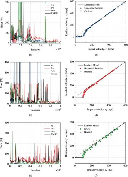
4.Conclusion

- Defence Technology的其它文章
- 3D laser scanning strategy based on cascaded deep neural network
- Damage analysis of POZD coated square reinforced concrete slab under contact blast
- Autonomous maneuver decision-making for a UCAV in short-range aerial combat based on an MS-DDQN algorithm
- The properties of Sn—Zn—Al—La fusible alloy for mitigation devices of solid propellant rocket motors
- The surface activation of boron to improve ignition and combustion characteristic
- Numerical investigation on free air blast loads generated from centerinitiated cylindrical charges with varied aspect ratio in arbitrary orientation