Machine learning-based method to adjust electron anomalous conductivity profile to experimentally measured operating parameters of Hall thruster

Andrey SHASHKOV,Mikhail TYUSHEV,Alexander LOVTSOV,Dmitry TOMILIN and Dmitrii KRAVCHENKO

JSC ‘Keldysh Research Center’,8 Onezhskaya St.,Moscow 125438,Russia

Abstract The problem of determining the electron anomalous conductivity profile in a Hall thruster,when its operating parameters are known from the experiment,is considered.To solve the problem,we propose varying the parametrically set anomalous conductivity profile until the calculated operating parameters match the experimentally measured ones in the best way.The axial 1D3V hybrid model was used to calculate the operating parameters with parametrically set conductivity.Variation of the conductivity profile was performed using Bayesian optimization with a Gaussian process(machine learning method),which can resolve all local minima,even for noisy functions.The calculated solution corresponding to the measured operating parameters of a Hall thruster in the best way proved to be unique for the studied operating modes of KM-88.The local plasma parameters were calculated and compared to the measured ones for four different operating modes.The results show the qualitative agreement.An agreement between calculated and measured local parameters can be improved with a more accurate model of plasma-wall interaction.

Keywords: Hall thruster,anomalous conductivity,machine learning,Bayesian optimization,Gaussian process,electric propulsion

1.Introduction

An increase in computational capacity promotes the application of numerical simulations to engineering design,and Hall thrusters are no exception.However,3D simulation of plasma dynamics in a Hall thruster is still a very computationally expensive task.Thus,until now,2D with three velocity space axisymmetric models(2D3V models)with the simulation region in the axial-radial plane (R-Z plane) [1,2] has practical significance in Hall thruster design.This is due to the shape of the simulation domain providing insight into the ceramic erosion intensity,the magnitude of the heat fluxes into construction,and the dependency of operating parameters on the thruster’s geometry.However,an axisymmetric simulation region excludes direct modeling of the electron transport driven by the growth of azimuthal instabilities [3-10].This electron transport is called‘a(chǎn)nomalous transport’in a variety of papers.At present,there is no self-consistent theory of anomalous transport that allows one to account for it in the R-Z plane.Additional elastic collision approximation is commonly used to simulate anomalous transport via existing numerical models.

The most widely seen approximation for anomalous transport is the Bohm effective collision model that suggests that the anomalous collisions are proportional to the electron Larmor frequency [11]:

whereνanois the frequency of the effective anomalous collisions,αis the proportion coefficient andcωis the electron cyclotron frequency.Many papers utilize the Bohm collision model due to its simplicity [12-20].However,this approximation yields an unfeasible distortion of the plasma layer location and causes the dependence of the plasma layer width on cathode boundary location [21].The reason for these uncertainties probably lies in a significant discrepancy of the anomalous collision distribution obtained in the experiment[4,22,23] and in the Bohm approximation.

The plasma-wall interaction is one of the possible mechanisms of electron transport across the magnetic field[24-28].However,classical electron conductivity supplemented by near-wall conductivity gives less additional current than necessary to explain the experimentally observed current.Thus,near-wall conductivity is at least not the only mechanism of the additional electron conductivity.

Some turbulent models describe the value of the anomalous transport based on first physical principles [29-31].In[32] the superposition of turbulent models from [29-31] was applied.The discharge channel was divided into three separate regions,each having its dominant transport model.The turbulent approach seems to be promising because of its apriority.However,the existing turbulent models use these input parameters as the magnitude or wave number of the resonant mode of plasma instability,which could not be obtained self-consistently from R-Z models.Consequently,the equation system with a turbulent model of electron transport still contains unknown or varied parameters.Currently,these unknown parameters are defined from experiment or independent calculations in R-θgeometry.

To date,the most accurate simulations have been conducted using experimental data about the anomalous conductivity function along the centerline of a Hall thruster[33,34].These data can be obtained via the laser-induced fluorescence (LIF) method [23],which entails rather expensive equipment that also demands special-purpose instrumentation of a vacuum chamber.

In an attempt to reduce the cost of the anomalous conductivity modeling,machine learning techniques were applied to generalize the data on the experimentally measured anomalous conductivity of some thrusters with discharge power ranging from 1-6 kW[35].The study yields the best-fit correlation between the anomalous conductivity along the centerline of the thruster and the local plasma parameters,such as ion axial and electron drift velocities.The obtained model is called the data-driven model of anomalous transport.However,when used in the Hall2De code [34],the obtained functional dependence gives a weak agreement between the modeled discharge current and experimental one [36] (the most probable discharge current value differed from the experimental one by 90%).Nevertheless,the authors took a big step towards the predictive model of anomalous conductivity.

In the observed papers,the problem to be solved was a direct one.In this work,we have tried to solve the inverse problem using the 1D3V hybrid model.The distribution of the anomalous conductivity along the centerline was the output parameter when the discharge current,thrust,plume divergence and beam energy homogeneity were the input parameters.The inverse problem could be solved either analytically,by applying the variation method,or numerically.In this work,we use the shooting method improved by machine learning techniques.The method is not predictive and does not give the exact solution.Therefore,the method does not apply to the engineering design of Hall thrusters.However,it provides a more feasible solution than the Bohm conductivity model and can be used for estimative calculations when LIF diagnostics is unavailable.

In section 2,we describe the experimental data that were used as the input parameters.Then,in section 3,the numerical model and system of equations are described.In section 4,we describe the algorithm used to solve the inverse problem and discuss whether the obtained solution is unique.The final section is devoted to discussion of the modeling results.

2.Experiment

The experimental data we refer to in this work are the results of measurements previously conducted in the Keldysh Research Center in vacuum chamber CVF-90[37].The study object was a laboratory model of a KM-88 Hall thruster with a centerline diameter of 88 mm and power of 1.5 kW[38].The goal of the procedure was to determine KM-88 thrust and discharge current.We also measured the thruster’s distribution of ion angular currentJ(θ,0)and its volt-ampere characteristicsJ(θ,U)with the help of a multi-grid probe located on the arc at a 150 cm distance from the thruster end and at a height aligned to the thruster axis.

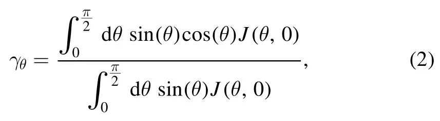
In [39],a method to calculate thruster efficiency parameters based onJ(θ,0)andJ(θ,U)was described.In particular,the angular deviation lossγθis written as,

and the rate of beam energy homogeneity took the following form:

whereγEis the rate of energy homogeneity andUdis the discharge voltage.The rate of energy homogeneity characterizes ion beam acceleration efficiency in the potential drop.WhenγEis equal to 100%,all the ions have been formed in the anode potential and have received energy equal to the discharge energy.The results of the measurements,which were later used in the simulations,are presented in table 1.

Table 1.Measurement results of the efficiency structure change in the KM-88a.

3.Numerical model

3.1.System of equations

Numerical simulations in this work were conducted using the updated 1D3V hybrid model described in [40].This allows one to consider neutrals and ion interactions with walls,charge exchange,secondary,step,double ionization,excitation and relaxation of the neutrals.Although the model permits one to account for a self-magnetic field of moving charged particles,we have omitted this option in the current work.The original numerically solvable set of equations for electron hydrodynamics is presented below.The continuity equation is written as,

Here,nis the electron concentration,ni+is the singly charged ion concentration,ni++is the doubly charged ion concentration,tis the time,zis the axial coordinate,νiis the ionization frequency.Uz+andUz++are the corresponding axial velocities of singly and doubly charged ions,β0,β1,β2andβ3-are the rate constants of single,double,secondary and stepwise ionization,respectively,andN* is the concentration of the excited neutrals.Excited atoms that relax with frequencyνrelax=107Hz [40] are considered in the kinetic part of the model.The value 107is an average between two de-excitations from the two first excited states with de-excitation coefficients3 ×107and2.7 ×106s-1.In this case,the ionization frequency is as follows:νi==β0N,ν1=2β1N,ν2=β2n,ν3=β3N*.

The momentum equation takes the following form:

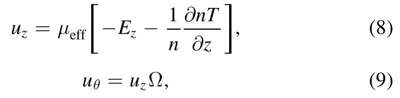
whereuzanduθare the electron velocities in the axial and azimuthal directions,respectively.The following notations are used:

whereEzis the axial part of the electric field,eis the elementary charge,Tis the electron temperature in volts,Ω is the Hall parameter,μeffis the effective mobility of the electrons,meis the electron mass,ωceis the cyclotron frequency of the electron rotation andνtotis the effective frequency of all collisions.Specific collision frequencies introduced above are as follows:eνis the electron momentum loss frequency,νexcitis the neutral excitation collision frequency,νelastis the frequency of the elastic collisions between electrons and neutrals,is the electron-ion Coulomb collision frequency,νewis the electron wall collision frequency andνanomis the effective anomalous collision frequency.Finally,Randrare the radii of the outer and inner walls of the discharge channel,respectively,Mis the xenon atom mass,Lis the length of the discharge channel andσis the secondary electron emission coefficient taken from the model from [18]:

The anomalous collision frequency set as the piecewise function was proposed in [41]:

wherezkdefines the segments of the anomalous collision frequency,fkare the proportionality coefficients between the frequency of the anomalous collisions and the electron Larmor frequency in half-interval∈[zk-1,zk);these coefficients range from 0-1,andkis the index from 1-6.Whenz＞z6,the anomalous collision frequency is calculated asνanom=f6ωce.

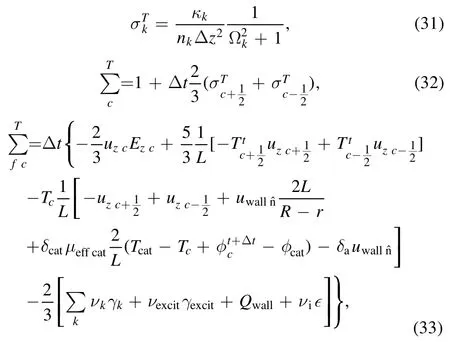
The temperature equation is written under the assumption that all non-diagonal stress tensor values are zero but still account for thermal conductivity of electrons across magnetic field lines:

where the parameter of thermal conductivity across magnetic field lines is defined from the expression of heat flux in the magnetic field [42] and written as,

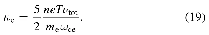
The heat flux to the wallQwallis described in the following subsection.

3.2.Simulation region,boundary conditions and initial conditions

The simulation region is an annular cylindrical channel with an inner radius of 35 mm,outer radius of 50 mm,centerline radius of 42.5 mm,channel length of 35 mm and simulation region length of 105 mm(see figure 1).The distance along the thruster axis is measured in dimensionless units,with the anode located at z=0 and the maximum of the magnetic field atzBmax=1.

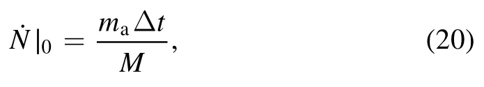
The boundary conditions for neutral gas are set at ceramic walls in the form of diffusive reflection with the temperature of the wall and at the anode in the form of a gas flow rate with the thermal velocity determined by the wall temperature:whereis the number of neutral atoms generated at the anode boundary per iteration,mais the anode gas flow rate andΔtis the time step.The temperature of the walls and anode was set to 600 K.The value was estimated via the increase in the resistance of the magnetic coils.

Boundary conditions for the charged plasma components are defined as follows.Ions are modeled kinetically and can recombine at walls and freely leave the simulation region through the right boundary.The ion flow to the ceramic walls is taken to be equal to the electron flow to these walls.The concentration of electrons at the boundaries is equal to the electron concentration in the border cell.The velocity of the normal electron flow to the walls is equal to the velocity of the Langmuir electron flow to a wall [43]:

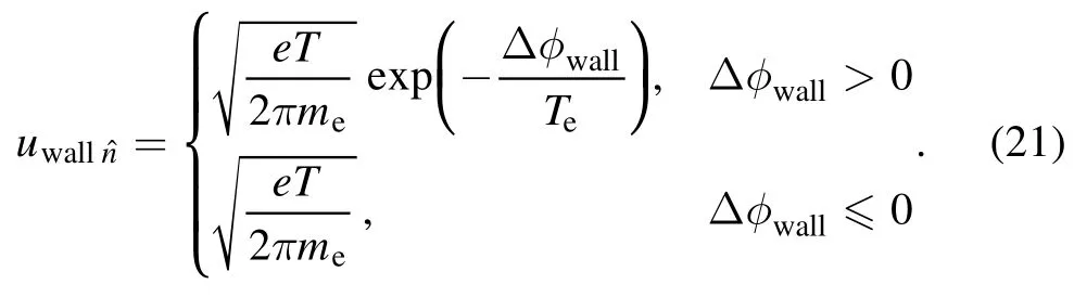
The potential drop at the wallΔφwallin the anode vicinity is determined as the difference between the plasma potential in the nearest cell and the anode potential.Potential drop at the ceramic boundaries is written as [43],

Heat flux to the wall is determined as,

and conductive heat flux to the wall is equal to zero.At the cathode boundary,the values of the cathode potentialφcat= 0and the electron temperatureTcat=3 eV are set.

As the initial condition for the first simulation in series,the simulation domain was filled with ion and neutral macroparticles uniformly distributed with a thermal velocity corresponding to the wall temperature,a linear drop of the potential from anode to cathode,and constant values for all electron parameters in the whole region.In addition,as the initial condition for future simulations in series,average profiles of all plasma parameters from the first simulation were used.

3.3.Difference scheme and computational grid

In this version of the model,to find the solution to the set of hydrodynamic equations,we used a first-order implicit method of finite volumes for time and space,whereas,in the previous version,it was an explicit first-order method of finite differences.The implicit method amplified the stability of the difference scheme and allowed one to take into account thermal conductivity in the equation for electron energy.

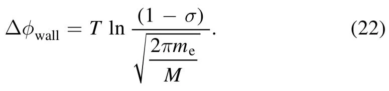
After integration of the equation set and the integral replacement with finite volumes,the difference scheme is written as,

with further notations:

Among the notations,jizis the ion flux in the axial direction,cis the index for the central cell that changes from 1 /2 toN-1 /2,andc±1 /2are the boundaries of the cells on each side.In this expression,the time index for the current step is omitted-only the indext+ Δtfor the next time step is left.

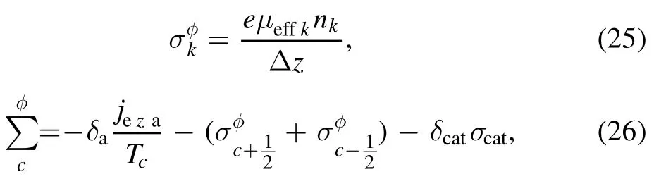
The equation on temperature is represented as,

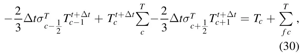
with the following notations introduced:

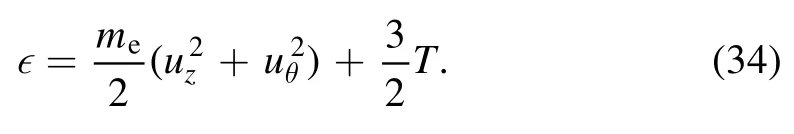
Both differential schemes were solved with the tridiagonal matrix algorithm.Interpolation from the center of each of the cells to their boundaries is linear:

3.4.Determination of the integral parameters

The average values for the operating parameters (thrust,discharge current and the rate of beam energy homogeneity)were determined after the simulation had become steady,namely when the current changed by less than 0.1%after ten ionization modes.Since the model is 1D,it was impossible to calculate the angular ion dispersion directly,possibly leading to an overestimated thrust value.To consider the angular dispersion of ions in a 1D model the thrust obtained in the simulations was multiplied by the experimentally measured angular loss coefficient

4.Method for the anomalous collision frequency determination

4.1.Selection criterion for the anomalous collision frequency

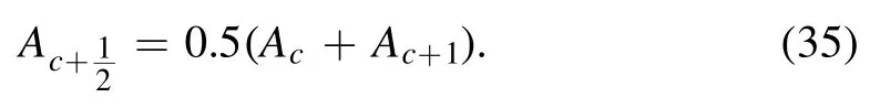
The 1D model described above allows one to receive operating thruster parameters,such as discharge current,thrust and beam energy homogeneity rate for a given profile of the anomalous collision frequency.In this work,we attempt to solve the inverse problem and find the anomalous collision frequency profile that meets operating parameters of the thruster obtained in the experiment (these parameters will be referred to as target parameters).Possible ways to derive a solution could either be ‘guessing’ (by mathematically shooting) the anomalous conductivity profile or applying algorithmic methods that use the information from previous calculations to refine the results at each step.The criterion determining the accuracy of the found solution will be referred to as the metric and is calculated by the following formula:

If the solution with the chosen anomalous collision frequency profile does not exist,the metric is equal to 10.Thereby,for any conductivity profile given by the formula(16),it is possible to determine the metric characterizing the deviation of the obtained solution from the target parameters.The anomalous conductivity function,which corresponds to the minimum of the metric in this method’s framework,is the desired function.

4.2.Metric minimization

Mathematically,the problem reduces to finding the minimum of the metric in the spaceG(fk,zk)with 2k dimensions.This function is not continuously differentiable onG.In addition,it is not smooth since the Monte-Carlo method is used to describe the heavy-particle collisions,and plasma parameters are averaged over an incomplete set of oscillatory periods.Figure 2 shows the calculated value of the metric for ten identical simulations carried out in a row.The noise dispersion,calculated by these ten simulations,is around 8.5% of the average value.

Figure 1.Simplified view of the simulation region.

Figure 2.Numerical noise for the metric function.

Figure 3.Results of BO work for the test task.

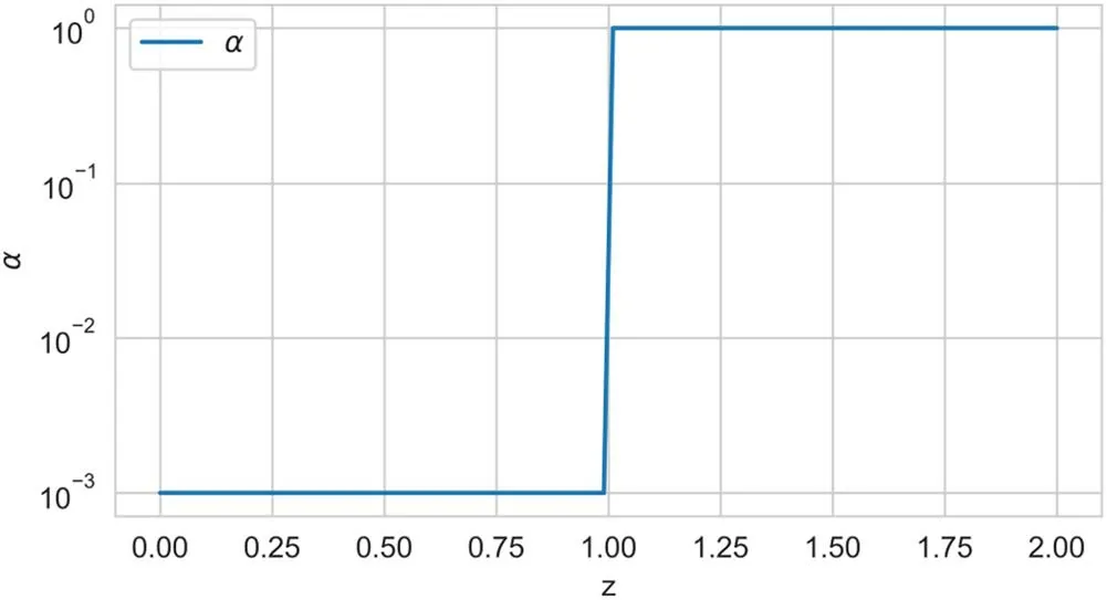
Figure 4.Form of the anomalous conductivity coefficient in the test task.

Figure 5.Dependence of (a) metric and target parameters [such as (b) thrust,(c) discharge current,(d) beam energy homogeneity rate] on variable parameters.

Therefore,methods of minimum search based on determining a function’s increment at a point,such as the gradient descent method,are hardly applicable.Finding the metric at a point in G takes around 10 min on a regular computer.This,along with the space G dimension,should be taken into account.Considering these factors,in this work,we propose to find the desired function via Bayesian optimization [44]with a Gaussian process [45].This method belongs to the family of machine learning methods that minimize the number of iterations needed to find a global minimum in spaces of high dimension that are not continuously differentiable.Herein,we exploit the numerical implementation of Bayesian optimization(BO)with Gaussian process gp_minimize()from the open-source library Scikit-Optimize [46].

4.3.Uniqueness of the solution

The main issue in solving this problem is the uniqueness of the anomalous conductivity profile,which corresponds to the target parameters.In other words,it is necessary to be sure that for each set of input parametersa unique set offk,zkexists,with the smallest possible metric.

Since BO finds all the minima that differ by a specified value from the global one,this shows all the minima the metric happens to have.A good demonstration of BO abilities is the test task,where the algorithm should find the minimum fory(x)=0.01x+ |1-x|at the intervalx∈ [-2,2].The graph for this function is shown in figure 3.The y function is not continuously differentiable at the given interval and has two minima: one is local (at the pointx=1 ),and another is global(at the pointx= -1 ).In the figure,the solid blue line shows the function itself.The black dots represent the results of the BO search,which do not exceed the valuey(1.05),and the red dot is the global minimum found by the BO.The test shows that the algorithm found all the minima and distinguished the global one among them,despite the lack of continuous differentiability.After 100 iterations,the algorithm achieved a 1.8% difference between the calculated and analytical minimum function value iny( -1).

We have verified the applicability of the BO algorithm to search for the metric minimum in the following way: the anomalous conductivity function was set with just two parametersf0andz0.With parameter valuesf0=10-3andz0= 1,the anomalous conductivity coefficient function takes the form shown in figure 4.The value of the anomalous conductivity coefficient atz＞z0did not change and was taken to be equal to 1.This assumption is very coarse yet possible since,in most works on anomalous conductivity measurements,the Hall parameter near the thruster cut is close to this value [42].

A series of simulations were conducted for different values off0andz0.The valuef0varied from 10-4to 6.1 ×10-3with step4 ×10-4,and the value forz0changed from 0.7 to 1.3 with a step of 0.04.For each pair of valuesf0andz0,the algorithm calculatedThe calculation of the metric for mode No.1 from table 1 builds upon these parameters.The obtained dependence helps to determine the range of the parametersf0andz0closest to the metric minimum.After that,we conducted a refining series of simulations with a four times smaller step for parametersf0andz0than in the first series.The received dependencies are shown in figure 5.Figure 5(c)shows that with a decrease inf0and an increase inz0(i.e.with a decrease in the integral conductivity in the anode region),the discharge current decreases.Figures 5(b) and (d) indicate the existence of this anomalous conductivity profile that allows one to obtain the maximum possible thrust and minimum possible losses on the beam energy homogeneity rate,respectively.Figure 5(a)shows that the final metric has a suitably long valley,where it only changes slightly and is close to the minimum value.Coupled with the metric noise (see figure 2),this fact complicates the search for the minimum with gradient-based methods.The metric’s minimum found with the grid method is equal to 0.0181,and its correspondingf0andz0are marked in figure 5 with a blue dot.

The valuesf0andz0corresponding to the metric minimum found by the BO method for mode No.1 from table 1 are depicted in figure 5 with a red dot and are equal to 0.0197.This value differs from the minimum found via the grid method by 7.8%.It is lower than the function noise of 8.5%.Taking into consideration that the minimum found through the grid method was obtained in a single calculation (that is,the noise can affect the position of this point),whereas the minimum discovered with BO includes this noise and is achieved in fewer iterations,the BO method successfully addresses the problem of finding the minimum.

If we were to approximate the anomalous conductivity function with more parameters (for example,with eight parameters as is the case later in this work),the grid method would not be applicable at all parameters due to its computational cost.

Figure 6 shows the comparison between the BO-found conductivity profiles specified by two and eight parameters.As can be deduced from the figure,the beginning of the anomalous conductivity drops for two and eight parameters are almost coincident.However,the conductivity shapes near the maximum of the magnetic field and in the anode region are different.In addition,the form of the anomalous conductivity profile found with eight parameters corresponds to the profile experimentally measured via LIF (figures 5 and 6 from [42],and figure 5 from [22]).

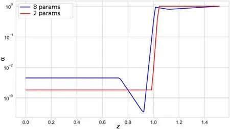
Figure 6.Measurement of the anomalous conductivity coefficient along the centerline for two and eight parameters.

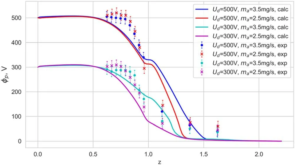
Figure 7.Comparison of plasma potential for different operating modes for KM-88 in simulations and experiment.

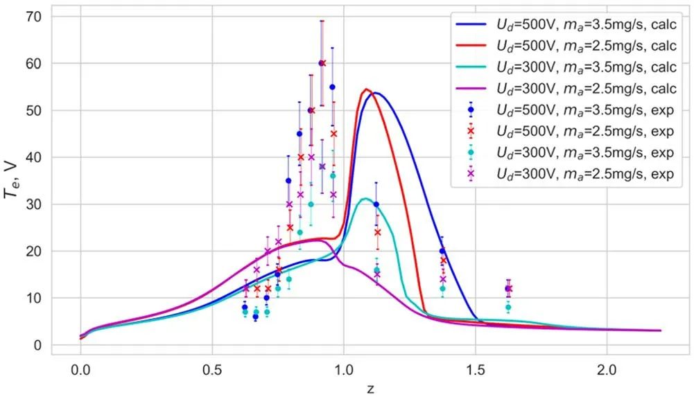
Figure 8.Comparison of electron temperature for different operating modes for KM-88 in simulations and experiment.

5.Results and their analysis

The modes introduced in table 1 were modeled with eight parameters for the anomalous conductivity profile using the BO method and 1D3V hybrid model.To validate the results,we used the data obtained from the wall probes in [37].Comparison of experimentally measured plasma potential profiles at the channel wall with calculation results at the channel centerline was made based on the assumption that magnetic field lines are equipotential[27].Error bars for these measurements are shown in the figures.The comparison is shown in figures 7 and 8.Notably,this comparison is only qualitative since it contains several substantive inaccuracies:(1) the 1D model does not and cannot take into account correctly the plasma-wall interaction,(2) the 1D model does not and cannot take into account the curvature of the magnetic field lines,which can gradually distort the anomalous conductivity profile in the anode region and influence the integral conductivity in the discharge gap.Nevertheless,this comparison has the qualitative agreement of the distributions obtained experimentally and numerically.

Figure 7 shows the distribution of the plasma potential.The width of the potential drop is in good agreement with the experimental result,although the layer location in the simulation is slightly shifted to the anode.Figure 8 shows the temperature distribution.An important point to note is the step on the figures near the channel exit (z=1).This step is caused by the influence of the plasma-wall interactions described in equation (14),and cannot be removed in 1D models.The same reason explains the difference in position between the temperature maxima in the experiment and the simulations in figure 8.Nevertheless,the model correctly predicts the shift in temperature profile due to a change in discharge voltage and gas consumption.In addition,the width of the temperature profile is quite close to that of the experiments.

Thus,the substantial possibility of obtaining the anomalous conductivity profile from the known integral parameters of the discharge has been shown.In the future,conductivity search can be performed with a 2D hybrid model on a rough grid to take into account heat fluxes to the discharge chamber walls,the curvature of the magnetic lines in the anode region,and the geometry of the discharge chamber (in the current setting,it is not possible to account for the widening of the discharge chamber close to the thruster cut).An undoubted advantage of the described method compared to the other methods based on measuring the anomalous conductivity profile is equipment accessibility.At the same time,in contrast to setting anomalous conductivity by the Bohm coefficient or a multi-zone model tied to the thruster’s geometry,this method allows one to observe how the conductivity transforms when one changes the gas consumption,the absolute value of the magnetic field or the discharge voltage.After replacing the 1D model with more accurate analogs,this method is applicable for simulating wall sputtering in the discharge chamber,studying physical processes and analyzing thruster test results.

6.Conclusion

In this work,we have proposed a method for determining anomalous conductivity in the Hall thruster channel based on machine learning and experimental data.It requires one to predetermine the operating parameters of the thruster,such as thrust,discharge current,angular divergence of the beam,and beam energy homogeneity rate.The accuracy of the method depends on the accuracy of the numerical model used for anomalous conductivity profile search.

A 1D3V hybrid model that can take into account the interaction between neutrals and discharge chamber walls was used.The fundamental possibility of implementing the proposed approach for the selection of the plasma anomalous conductivity along the centerline was demonstrated using the developed model.The accuracy of the plasma potential and electron temperature distribution obtained via the 1D model can be further increased with more accurate numerical models.