
A Level Set Representation Method for N-Dimensional Convex Shape and Applications
2021-05-13 11:07:34LingfengLiShoushengLuoXueChengTaiandJiangYang
Lingfeng Li,Shousheng Luo,Xue-Cheng Tai and Jiang Yang
1 Department of Mathematics of Hong Kong Baptist University,Hong Kong,SAR,China.
2 Department of Mathematics of Southern University of Science and Technology,Shenzhen,China.
3 School of Mathematics and Statistics,Henan Engineering Research Center for Artificial Intelligence Theory and Algorithms,Henan University,Kaifeng,China.
Abstract.In this work,we present a new method for convex shape representation,which is regardless of the dimension of the concerned objects,using level-set approaches.To the best of our knowledge,the proposed prior is the first one which can work for high dimensional objects.Convexity prior is very useful for object completion in computer vision.It is a very challenging task to represent high dimensional convex objects.In this paper,we first prove that the convexity of the considered object is equivalent to the convexity of the associated signed distance function.Then,the second order condition of convex functions is used to characterize the shape convexity equivalently.We apply this new method to two applications:object segmentation with convexity prior and convex hull problem(especially with outliers).For both applications,the involved problems can be written as a general optimization problem with three constraints.An algorithm based on the alternating direction method of multipliers is presented for the optimization problem.Numerical experiments are conducted to verify the effectiveness of the proposed representation method and algorithm.
Key words:Convex shape prior,level-set method,image segmentation,convex hull,ADMM.
1 Introduction
In the tasks of computer vision,especially image segmentation,shape priors are very useful information to improve output results when the objects of interest are partially occluded or suffered from strong noises,intensity bias and artifacts.Therefore,various shape priors are investigated in the literature[5,14,20,33].In[8,20],the authors combined shape priors with the snakes model[2]using a statistical approach and a variational approach,respectively.Later,based on the Chan-Vese model[5],a new variational model,which uses a labeling function to deal with the shape prior,was proposed in[11].A modification of this method was presented in[4]to handle the scaling and rotation of the prior shape.All the priors used in these papers are usually learned or obtained from some given image sets specifically.
Recently,generic and abstract shape priors have attracted more and more attention,such as connectivity[36],star shape[34,39],hedgehog[18]and convexity[15,33].Among them,the convexity prior is one of the most important priors.Firstly,many objects in natural and biomedical images are convex,such as balls,buildings,and some organs[30].Secondly,convexity also plays a very important role in many computer vision tasks,like human vision completion[23].Several methods for convexity prior representation and its applications were discussed in the literature[14,33,38].However,these methods often work for 2-dimensional convex objects only and may have relatively high computational costs.In this paper,we will present a new method for convexity shape representations which is suitable for high dimensional objects.
Most of the existing methods for convex shape representation can be divided into two groups:discrete approaches and continuous approaches.For the first class,there are several methods in the literature.In[31],the authors first introduced a generalized ordering constraint for convex object representation.To achieve the convexity of objects,one needs to explicitly model the boundaries of objects.Later,an image segmentation model with the convexity prior was presented in[14].This method is based on the convexity definition and the key idea is penalizing all 1-0-1 configurations on all straight lines where 1(resp.0)represents the associated pixel inside(resp.outside)the considered object.This method was then generalized for multiple convex objects segmentation in[13].In[30],the authors proposed a segmentation model that can handle multiple convex objects.They formulated the problem as a minimum cost multi-cut problem with a novel convexity constraint:If a path is inside the concerned object,then the line segment between the two ends should not pass through the object boundary.
The continuous methods usually characterize the shape convexity by exploiting the non-negativity of the boundary curvature in 2-dimensional space.As far as we know,the curvature non-negativity was firstly incorporated into image segmentation in[33].Then,a similar method was adopted for cardiac left ventricle segmentation in[38].In[1],an Euler’s Elastica energy-based model was studied for convex contours by penalizing the integral of absolute curvatures.Recently,the continuous methods or curvature-based methods were developed further in[24,37].For a given object in 2-dimensional space,it was proved in[37]that the non-negative Laplacian of the associated signed distance function[32](SDF)is sufficient to guarantee the convexity of shapes.In[24],the authors also proved that this condition is also necessary.Also,instead of solving negative curvature penalizing problems like[1,33,38],these two papers incorporated non-negative Laplacian condition as a constraint into the involved optimization problem.This method has also been extended for multiple convex objects segmentation in[25].Projection algorithm and the alternating direction method of multipliers(ADMM)were presented in[24,37].
In some real applications,one needs to preserve the convexity for high dimensional objects,such as tumors and organs in 3D medical images.Therefore,it is very significant to study efficient representation methods for high dimensional convex objects.However,there are some difficulties in theories and numerical computation for the existing methods mentioned above to be generalized to higher dimensions.
For the discrete methods in[15,30],it is almost impossible to extend these methods to higher dimensional(≥3)cases directly because of the computational complexity.One can set up the same model as the two-dimensional case,but the computational cost will increase dramatically.For the continuous methods using level-set functions[24,33],the mean curvature(Laplacian of the SDF)of the zero level-set surface can not guarantee the convexity of the object convexity in high dimensions.For example,in the 3-dimensional space,an object is convex if and only if its two principal curvatures always have the same sign at the boundary.Accordingly,one should use the non-negativity of Gaussian curvatures to characterize the convexity of objects[12].However,the problems(e.g.,optimization problems for image segmentation)with non-negative Gaussian curvature constraint or penalty are very complex and difficult to solve.As far as we know,there is no existing method that can characterize the convexity of high dimensional objects.
In this work,we present a new convexity prior which works in any dimension.Similar to the framework in[24],we also adopt the level-set representations,which is a powerful tool for numerical analysis of surfaces and shapes[26,27,40]and have many applications in image processing[3,22,35].We first prove the equivalence between the object convexity and the convexity of the associated SDF.It is well-known that a convex function must satisfy the second-order conditions,i.e.,having positive semi-definite Hessian matrices at all points if it is secondly differentiable.Based on this observation,we obtain a new way to characterize the shape convexity using the associated SDF.The proposed methods have several advantages.Firstly,it works regardless of the object dimensions.Secondly,this method can be easily extended to multiple convex objects representation using the idea in[25].Thirdly,this representation is simple and tractable.
To verify the effectiveness of the proposed method,we apply it to two applications in computer vision and design algorithms to solve them.The first one is the image segmentation task with convexity prior[15,24,33].More specifically,we combine the convexity representation with a 2-phase probability-based segmentation model.The second model is the variational convex hull problem,which was first introduced in[21]for 2-dimensional binary images.This model can compute multiple convex hulls of separate objects simultaneously and is very robust to noises and outliers compared to traditional methods.However,since it uses the same convexity prior with[24],it works only for 2-dimensional problems.Using the proposed method,we can generalize it to higher dimensions and maintain all of its advantages,e.g.,robustness to outliers.
Both applications can be formulated as a general constrained optimization problem.Similar to[21,22,24],the alternating direction method of multiplier(ADMM)for the general optimization problem is derived to solve the models.In the proposed algorithm,the solutions of all sub-problems can be derived explicitly or computed relatively efficiently.Numerical results for the two concerned problems are presented to show the effectiveness of our convexity prior.
The rest of this paper is organized as follow.In Section 2,we will introduce some basic notations and results from convex optimization.Then we will present the convexity prior representation method in Section 3.Section 4 is devoted to two variational models for the two applications.The numerical algorithm will then be given in Section 5.In Section 6,we will present some experimental results in two and three-dimensional spaces to test our proposed methods.Conclusions and future works will be discussed in Section 7.
2 Preliminaries
First,we will briefly introduce some results from convex optimization in this section.Given a set of pointsin Rd,a point in the formis called a convex combination of {xi} if θi≥0 and.Then,given a set C in Rd,it is said to be convex if all convex combinations of the points in C also belong to C.The convex hull or convex envelope of C is defined as the collection of all its convex combinations,i.e.,
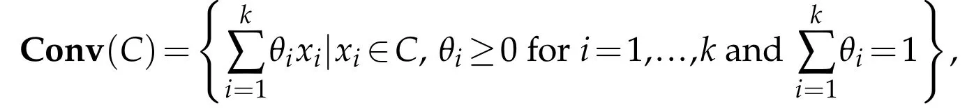
where k can be any finite positive integer.In other words,Conv(C)is the smallest convex set containing C.
Another important concept is the convex function.Given a function f(x):Rd→R∪{+∞},f(x)is a convex function if its epigraph{(x,f(x))|x∈Rd}is a convex set.If f is twice differentiable,a necessary and sufficient condition for the convexity is that the Hessian matrix of f is positive semi-definite at every x,i.e.

where H f(x)denotes the Hessian matrix of f at x.
For any measurable f and real numberα,we can define theαlevel-set,α sublevel-set andαsuperlevel-set of f as follow:
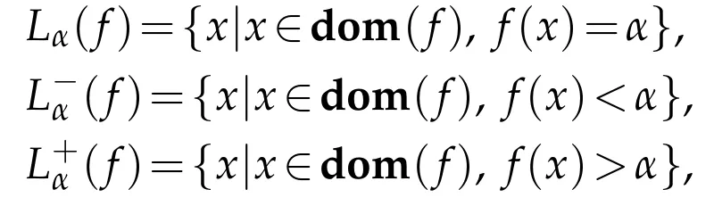
wheredom(f)denotes the domain of f.It is easy to verify that if f(x)is convex,(f)is also convex for anyα∈R.
Next,we are going to introduce a powerful tool,named level-set function,for the implicit representation of shapes.Given an open setΩ1in Rdwith piecewise smooth boundaryΓ,the level-set function,denoted asφ(x):Rd→R,ofΓsatisfies:

whereΩ0is the exterior ofΓ.We further assume thatΩ1is nonempty andΓ has zero measure in the rest of this paper.Equivalently,we can also denoteΩ1as(φ),Γas L0(φ)andΩ0as(φ).Then,the evolution of the hypersurfaceΓcan be represented by the evolution ofφimplicitly.The main advantage of the levelset method is that it can track complicated topological changes and represent sharp corners very easily.Using the heaviside function h(·),we can obtain the characteristic function of Ω0by h(φ(x))and the characteristic function ofby 1-h(φ(x)).The distributional derivative of the heaviside function is denoted asδ.
In this work,we are going to use the signed distance function,which is a special type of level-set function,to represent convex shapes.For an open set Ω1with piecewise smooth boundaryΓ,the SDF ofΓis defined as


where the gradient is defined in the weak sense.Notice that the weak solution of(2.2)is not unique,but one can define a unique solution in the viscosity sense[10]given certain boundary conditions.We also obtained an interesting property for the SDF:
Lemma 2.1.Suppose we are given two compact subset C1and C2in Rd.Denotes their boundaries by Γ1and Γ2,and their SDFs by φ1and φ2,respectively.Thenif and only if φ1(x)≥φ2(x) for any x.
The proof of this result will be given in the next section.This result is very useful in computing the convex hull via level-set representation.
In[24],the authors presented an equivalent condition of 2-dimensional object convexity

whereφis the associated SDF.It can be shown that Δφ(x)equals to the mean curvature of the level-set curve Lc(φ)at the point x,whereφ(x)=c.In the twodimensional space,if the mean curvatures of the zero level-set curves are nonnegative,the object Ω1must be convex.However,this is not the case in higher dimensions.
3 Convexity representation for high dimensional shapes
In[24],the authors proved that a 2-dimensional shape is convex if and only if any sublevel-set of its SDF is convex.One can show that the convexity of a shape is also equivalent to the convexity of its SDF and this is true in any dimensions.We summarize this result in the following theorem.
Theorem 3.1.LetΓbe the boundary of a bounded open convex subsetΩ1?Rdandφbe the corresponding SDF of Γ.Then,Ω1is convex if and only if φ (x)is convex.
It is well-known that the SDFφmust satisfy the second-order condition(2.1)if it is secondly differentiable.Therefore,we can use the condition(2.1)to represent the convexity of shapes.Before proving Theorem 3.1,we need to introduce some useful lemmas.
Lemma 3.1.LetΓbe the boundary of a bounded open convex subsetΩ1?Rdandφbe the corresponding SDF ofΓ.For any x inthere exists a unique Px∈Γsuch that

In other words,the projection of an exterior point must belong to Γ.
Actually,one can generalize this result to non-convex Ω1without difficulty.The next lemma can be directly derived from the definition of SDF.
Lemma 3.2.LetΓbe the boundary of an open subset Ω1?Rdandφbe the corresponding SDF of Γ.Then for any elementand non-negative c,the inequality φ(x)≤-c is true if and only if B(x,c),where B(x,c)={z∈Rd|‖z-x‖2<c}.
A simple corollary of the Lemma 3.2 is thatfor any x∈.Now,we can give the proof of Theorem 3.1 as follows:
Proof.We first assumeΩ1is convex.Let x1and x2be any two elements in Rdand x0=θ x1+(1-θ)x2.We would like to show thatφ(x0)≤θ φ(x1)+(1-θ)φ(x2)for anyθ∈[0,1].We will divide the proof into three parts.
(i)First,if x1and x2are ini.e.,φ(x1)≥0 andφ(x2)≥0.By Lemma 3.1,there exist unique y1∈Γand y2∈Γsuch thatφ(x1)=‖x1-y1‖2andφ(x2)=
‖x2-y2‖2.If x0∈Ω0,let y0=θy1+(1-θ)y2∈Ω1,and we have

If x0∈,we haveφ(x0)≤0≤‖x0-y0‖2.
(ii)If x1and x2are in,then x0is also inΩ1.Let r=θ|φ(x1)|+(1-θ)|φ(x2)|.

Then,we can rewrite y as y=θ(x1+v1)+(1-θ)(x2+v2).Since

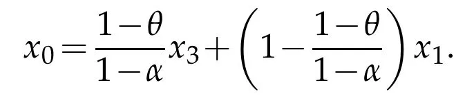
(iii)If x1∈Ω1and x2∈Ω0,there exists a Px2∈Γsuch thatφ(x2)=‖x2-Px2‖2.
By the continuity ofφ,there exists an x3=αx1+(1-α)x2,whereα∈(0,1),φ(x3)=0,and x0∈Ω0for anyθ<α.Denote y0=αx1+(1-α)Px2∈.We can compute that

By(ii),we have

Consequently,we have 0=φ(x3)≤αφ(x1)+(1-α)φ(x2).For any 1≥θ>α,x0=θ x1+(1-θ)x2∈,and then
Since x0and x1are in,we know that

If 0≤θ<α,we can similarly derive that

Based on(i),(ii) and (iii),we can conclude that φ(x0)≤θ φ(x1)+(1-θ)φ(x2)for any x1and x2in Rd.Conversely,ifφ(x)is convex in Rd,by the definition of convex function,all the sublevel-sets ofφare convex,so is
We have already proved that for any convex shapeΩ1,its corresponding SDF φmust be a convex function.Consequently,φmust satisfy the second-order condition where it is secondly differentiable.Note that a SDF usually is non-differentiable at a set of points with zero measure,so the second-order condition holds almost everywhere in the continuous case.In the numerical computation,since we only care about the convexity ofΓ,to save the computational cost,we can only require the condition holds in a neighbourhood around the object boundary,i.e.,

for some∈>0.
Lastly,using the Lemmas 3.1 and 3.2,we can prove Lemma 2.1 as follows:
Proof.Suppose C1?C2,then we would like to show thatφ1(x)≥φ2(x)for any x∈Ω.If x∈ΩC2,by Lemma 3.1,we have

If x∈C2but x/∈C1,then φ1(x)≤0≤φ2(x).If x∈C1,by Lemma 3.2,then we have

There fore,we can conclude that φ1(x)≥φ2(x)in Rd.
Conversely,if φ1(x)≥φ2(x)in Ω,for any x∈C1,φ2(x)≤φ1(x)≤0 which implies that C1?C2.
4 Two variational models with convexity constraint
In this section,we will present the models for two applications involved convexity prior in details using the proposed convexity representation method.
4.1 Image segmentation with convexity prior
Given a digital image u(x)∈{0,...,255}defined on a discrete image domain,the goal of image segmentation is to partition it into n disjoint sub-regions based on some features.To achieve this goal,many algorithms have been developed in the literature.Here we consider a 2-phase Potts model[28]for segmentation:

where fjis the corresponding region force term of each class andis the regularization term of the class boundaries.In the 2-phase case,usually is the object of interest and?Ω0is the background.
In this paper,we want to consider the segmentation problem with the convexity prior,i.e.,the object is known to be convex.Using the level-set representation and the results in the previous section,we can write the concerned segmentation problem as

where h(·)denotes the Heaviside function and g(x)=α/(1+β|?K*u(x)|)is an edge detector.K denotes a smooth Gaussian kernel here.The first unitary gradient constraint can maintainφto be a SDF and the second constraint is the convexity constraint.Since we only care about the convexity of the zero level-set,we can only impose this constraint in a neighbourhood around the zero level-set to save the computational time.
There are many ways to define the data terms f1and f0.In this work,we choose to use a probability-based region force term as in[24],where the data terms are computed from some prior information.Suppose we know the labels of some pixels as prior knowledge,then we denote I1as the set of labeled points belonging to phase 1 and I0as the set of labeled points belonging to phase 0.Define the similarity between any two points inΩas

where we will set a=1 and b=10 in this work.Then,the probability of a pixel x belonging to phase 1 can be computed as

and the probability belonging to phase 0 is p0(x)=1-p1(x).The region force term is then defined as fi(x)=-log(pi(x)),i=1,2.One can refer to[24]for more details about the segmentation model.Therefore,the model(4.1)can be rewritten as
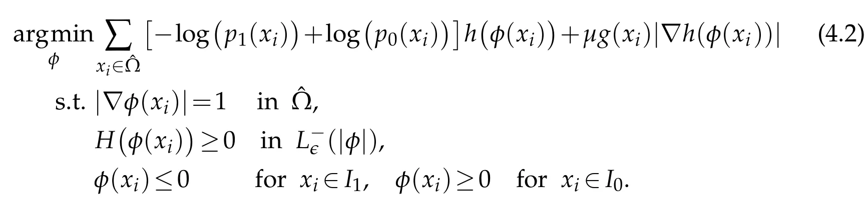
The numerical discretization scheme for the differential operators?(·)and H(·)will be introduced later in Section 5.Similar to[21],we assume that the input image u is periodic in Rdwhich implies thatφsatisfies the periodic boundary condition on?Ω.Using the fact that|?h(φ)|=δ(φ)|?φ|=δ(φ),the last term in the objective functional can be written as g(x) δ (φ(x)) where δ(·) is the Dirac delta function.In the numerical computation,we will replace h(·)andδ(·)by their smooth approximations

whereαis a small positive number.The segmentation model(4.2)can also be directly generalized to high dimensional cases for object segmentation.
4.2 Convex hull model
Suppose we are given a hyper-rectangular domainΩ?Rdand we want to find the convex hull of a subset X?Ω.From the definition,we know that the convex hull is the smallest convex set containing X.If we denote the set of all SDFs of convex subset inΩas K,the SDF corresponding to the convex hull minimizes the zero sub-level set area(or volume)among K

By Lemma 2.1,we can obtain an equivalent and simpler form

which leads to the following discrete problem:

This model is a simplified version of the convex hull models in[21]and can be applied to any dimensions.Here the first two constraints are the same with the segmentation model(4.2).The last constraint requires the zero sublevel-set ofφ contain X.Again,we assumeφsatisfies the periodic boundary condition.
As we mentioned before,when the input data contains outliers,it is not appropriate to requireto enclose all the given data in X.Instead,we can use a penalty function R(x)to penalize largeφ(x)for all x∈X.By selecting appropriate parameters,we can find an approximated convex hull of the original set with high accuracy.The approximation model is given as

where m(x)equals 1 in X and 0 elsewhere.Here we can choose R to be the positive part function

or its smooth approximation

for some t>0.
5 Numerical algorithm
Here we propose an algorithm based on the alternating direction method of multipliers(ADMM)to solve the segmentation model(4.2)and the convex hull models(4.3)-(4.7).We will also introduce the discretization scheme for the differential operators.
5.1 ADMM algorithm for the segmentation model and convex hull models
First,we write the three models(4.2),(4.3)and(4.7)in a unified framework:
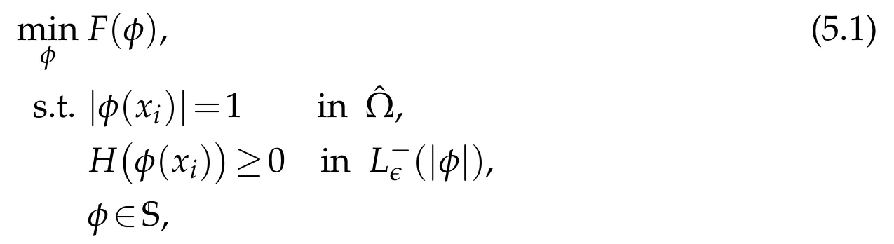
where F(φ)could be the objective functional in(4.2),(4.3)or(4.7),and S is defined as

For the segmentation model(4.2),I0and I1are those labelled points.For the exact convex hull model(4.3),I0is the set X and I1is empty.For the approximate convex hull model(4.7),both I0and I1could be empty.If we have any prior labels for the approximate convex hull model,we can also incorporate them into the models to make I0and I1non-empty.
To solve model(5.1),we introduce three auxiliary variables p=?φ,Q=H(φ),and z=φ.Then we can write the augmented Lagrangian functional as

with the following constraints:

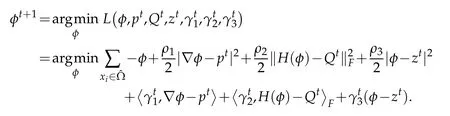
where S is specified by the problem at hand.Applying the ADMM algorithm,we can split the original problem into several sub-problems.
1.φsub-problem:
Then the optimalφmust satisfy

where?*(·)is the adjoint operator of?(·)and H*(·)is the adjoint operator of H(·).It is equivalent to
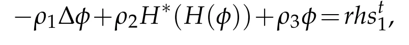

where

is a constant vector here.Sinceφsatisfies the periodic boundary condition,we can apply FFT as[21]to solve it.
2.p sub-problem:

3.Q sub-proble m:

The computation of this projection is very simple and can be done by the same way with[29].Given a real symmetric matrix A∈Rn×n,suppose its singular value decomposition is A=QΛQT,where Q is orthonormal and Λ=diag(λ1,...,λn)is a diagonal matrix with all the singular values of A on its diagonal entries.If we define

then the projection of A onto the set of all symmetric positive semi-definite(SPSD)matrices under the Frobenius norm is A*=QΛ+QT.The proof can be found in[17].
4.z sub-problem:

We summarize this procedure in Algorithm 1.
5.2 Numerical discretization scheme
Suppose we are given a volumetric data I∈RN1×···×Ndwhich is a binary function defined on the discrete domainΩh.I can also be viewed as a characteristic function of a subset Xh?Ωh.Each mesh point inΩhcan be represented by a d-tuple
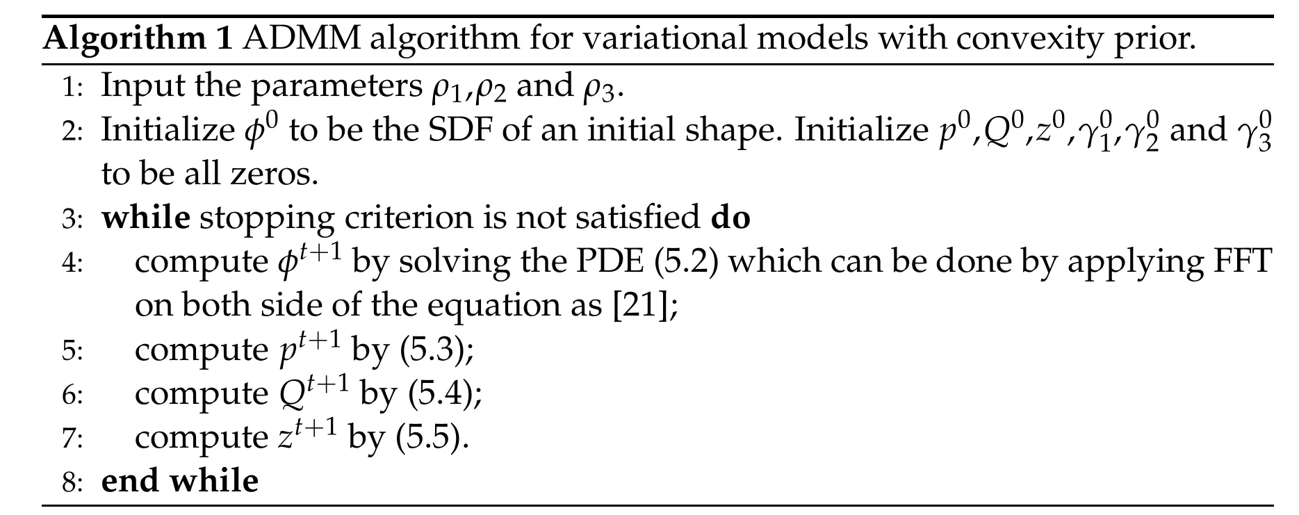
Algorithm 1 ADMM algorithm for variational models with convexity prior.1:Input the parametersρ1,ρ2 andρ3.2:Initializeφ0 to be the SDF of an initial shape.Initialize p0,Q0,z0,γ01,γ02 andγ03 to be all zeros.3:while stopping criterion is not satisfied do 4:computeφt+1 by solving the PDE(5.2)which can be done by applying FFT on both side of the equation as[21];5:compute pt+1 by(5.3);6:compute Qt+1 by(5.4);7:compute zt+1 by(5.5).8:end while
x=(x1,...,xd)where xiis an integer in[1,Ni]for i=1,...,d.To compute the convex hull of Xhusing the algorithm described before,we need first to approximate the differential operators numerically.For any functionφ:Ωh→RN1×···×Nd,we denot e(x)and(x)as

These are exactly the standard forward difference and backward difference.Then we approximate the first and second order operators as follow:
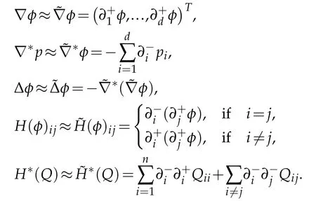
One can verify that the relationis also preserved by this discretization scheme.
6 Numerical experiments
In this section,we are going to demonstrate some numerical experiments of the segmentation models and convex hull models.The main purpose of these experiments is to show that our prior can guarantee the convexity of concerned objects accurately,especially in high dimensional cases.Due to the lack of studies in this area before,we do not make extensive comparisons with other methods.
6.1 Image segmentation and object segmentation
We first test our segmentation model for some images from[24].In Fig.1,we test the segmentation model(4.2)on a tumor image(a).Since the model needs some prior information,we give the prior labels in(b)and the initial curve in(c).One can observe that there exists a dark region in this tumor.If we do not impose the convexity constraint,the result we get is shown in(d),where the dark region is missing.After imposing the convexity constraint,we can recover the whole tumor region.The result of our algorithm is shown in(f)which is very similar to the result in[24](e).

Figure 1:Segmentation results of a tumor with and without convexity constraint.
We also test the segmentation model on 3D data of brain tumor from[19].The size of this volume is 240×240×152.In Fig.2,we show some cross-sections of the original volume.Then we give some prior labels at these 9 slices as in Fig.3 to compute the region force term.The initial region is taken as the set where the region force is positive.One can observe that the initial region shows some concavity in several slices,e.g.,z=90.We then compute the segmentation result using our proposed method.The 3-d visualization of the segmentation result is shown in Fig.5 and some cross-sections are presented in Fig.6.Though the initial shape is not convex,we can see that the convexity method can obtain a convex shape.What is more,the tumor region is also identified accurately.

Figure 2:Original 3-D volume of a brain tumor.

Figure 3:Prior labels assigned for the tumor.Red points represent foreground labels and yellow points represent background labels.

Figure 4:Some cross sections of the initial shape for the model.The initial shape is the set of points at which the region force term is positive.

Figure 5:Different views of the 3D visualization of the tumor.
6.2 Convex hull model
We first conduct experiments on 3-dimensional shapes from the ShapeNet dataset[6].The original object and computed convex hulls are shown in Figs.7 and 8.For this set of experiments,we useand∈=10.We also plot some level-set surfaces of the computed SDF in Fig.10.For all the level-set surfaces up to 10,they are convex,since we require the Hessian matrix is PSD in L10(|φ|).When we look at the 15-level-set surfaces,we can easily find concavity.We also compute the relative error[21]compared to a benchmark result obtained by the quickhull algorithm.The error of the chair and table objects are 5.18%and 4.31%,respectively.Moreover,we use the previous convexity prior[21]to compute the convex hull(Fig.9)and it can be observed that the obtained results are not convex at all,which is not surprising.

Figure 6:Different cross sections of the segmentation result of the brain tumor.

Figure 7:Convex hull of a chair.The first row shows the original volumetric data and the last two rows show different views of the convex hull.

Figure 8:Convex hull of a table.The first row shows the original volumetric data and the last two rows show different views of the convex hull.

Figure 9:Convex hull result using the previous convexity prior which cannot guarantee the convexity for 3d objects.
Then,an experiment with multiple objects has also been conducted.When there is more than one object in the given volume,we may be interested in obtaining convex hulls for each object separately.If we use some conventional methods to do this,we may need some object detection algorithm to extract the region of each object first.However,in our algorithms,we can achieve this by selecting a small∈value.Recall that the convexity constraint we imposed is that H(φ)≥0 in L∈(|φ|).The SDF of multiple convex hulls is convex only in a small neighborhood around each object.As long as our∈is small enough,our algorithm will return the separated convex hulls of each object.More specifically,∈should be smaller than half of the distance between each pair of objects.The numerical results are shown in Fig.11.We use the same set of parameters with the previous experiment here.From the result,we can see that when∈=5,our exact algorithm can compute the separated convex hulls accurately.When we set∈=20,we can get the big convex hull containing two cars together.We also plot the level-set surfaces to further illustrate how it works in Fig.12.When∈=5,we plot the 5 and 20 level-set surfaces.We can observe that the 5 level-set consists of two separated surfaces and both of them are convex.If we look at the 20 level-set surface,it is non-convex at somewhere between two cars.Since we only require H(φ)≥0 in L5(|φ|),the non-convexity on the 20 level-set does not violate the constraint.

Figure 10:Different level-set surfaces.Here we plot the 0,5,10 and 15 level-set surfaces of the computed SDFs.The first row is for the chair object and the second row is for the table object.

Figure 11:Convex hulls of multiple objects.The first column shows the original data of two cars.The second column is the convex hulls when setting∈=5 and the third column is the convex hull when setting∈=20.
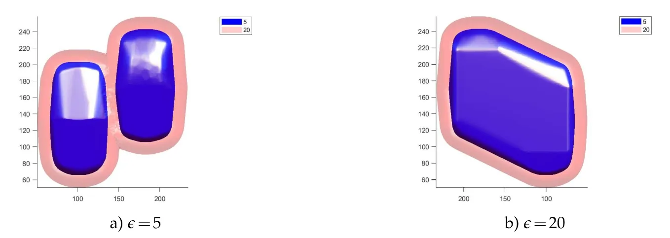
Figure 12:Level-set surfaces of the corresponding SDF when∈=5 and∈=20.
However,if we set∈=20,this SDF is not feasible anymore and what we will get is the SDF in(b)which corresponds to the convex hull of two cars combined.
As demonstrated in[21],the variational convex hull algorithm is very robust to noise and outliers.In 3-dimensional cases,the model can still preserve this advantage after applying our proposed prior.We choose two objects from the shape-net dataset[6]and generate some outliers,which are randomly sampled from a uniform distribution to the volumetric data.The approximate results are shown in Figs.13 and 14.The parameters we used in this experiments isρ0=400,ρ2=2000,ρ1==800 and∈=5.
We can observe that even if there exist large amount of outliers in the input,our algorithm can still obtain a very good approximation to the original convex hull.We also compare our result with the convex layer methods[7],which is also called the onion peeling method.Though many convexity priors have been proposed in recent years[14,15,24,30,36],they only work for 2d images,so we can only compare our method with relatively old methods.Given a finite set of points X,the convex hull of X is called the first convex layer.Then,we remove those points on the boundary of Conv(X)and compute the convex hull for the rest points.The new convex hull is called the second convex layer.By continuing the same procedure,we can get a set of convex layers and each point in X must belong to one layer.The convex layer method for outliers detection usually relies on two assumptions[16].Firstly,the outliers are located in the first few convex layers.In other words,the outliers are evenly distributed around the object.Secondly,the approximate number of outliers is known,which is not easy to obtain in some situations.We briefly described a convex layer algorithm for convex hull approximation in Algorithm 2.

Figure 13:Convex hull of a camera with some outliers.

Figure 14:Convex hull of a headphone with some outliers.

Algorithm 2 Convex layer method for convex hull approximation.1:Input a set of points X and the estimated number of outliers k,where k should be smaller than|X|.2:Set count=0.3:while count<k do 4:Compute the convex hull of X.5:Set CX be the set of points lying on the boundary of Conv(X).6:Delete points in CX from X.7:count=count+|CX|.8:end while 9:Return Conv(X)as the approximated convex hull.
For the camera and the headphone objects,the estimated number of outliers K are set to be 1400 and 2300,and the exact number of outliers are 1371 and 2268 respectively.From the results of the convex layers method in Fig.15,we see that even a very accurate k is given,the approximate convex hulls still deviate a lot from the true solution.Looking at the error in Table 1,our method beats the convex layer method by a huge margin.
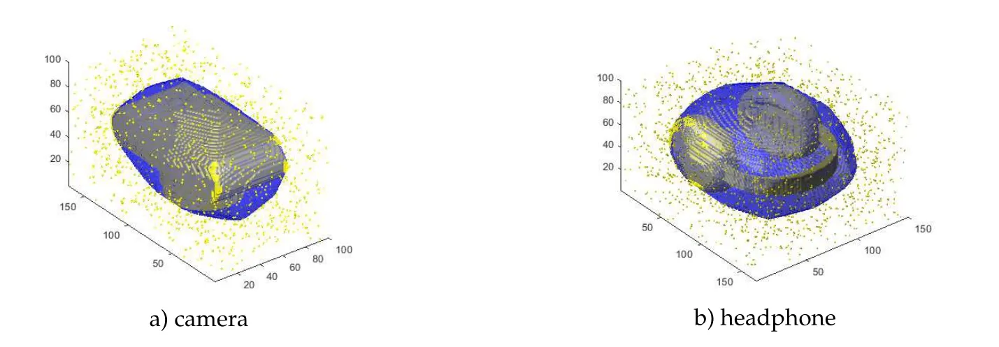
Figure 15:Approximate convex hulls by the convex layer method.

Table 1:The relative errors of our method and the convex layers method.
7 Conclusions and future works
In this work,we presented a novel level-set based method for convexity shape representation in any dimensions.To the best of our knowledge,this is the first representation method for high dimensional 3D shapes.The method uses the second-order condition of convex functions to characterize the convexity.We also proved the equivalence between the convexity of the object and the convexity of the associated SDF.This new method is very simple and easy to implement in real applications.Two applications with convexity priors in computer vision were discussed and an algorithm for a general optimization problem with the proposed convexity prior constraint was presented.Experiments for two and three-dimensional examples were conducted and presented to show the effectiveness of the proposed method.During the ADMM iteration,most of the computational effort is spent on the SVD for the Hessian matrices,which increases the computational time a lot.In future research,we will devote our effort to design a more efficient algorithm for our models.We will also explore more potential applications of our convexity prior,especially in high dimensional spaces,and other representation methods for generic shapes.
Acknowledgments
The work of Xue-Cheng Tai was supported by RG(R)-RC/17-18/02-MATH,HKBU 12300819,and NSF/RGC grant N-HKBU214-19 and RC-FNRA-IG/19-20/SCI/01.Shousheng Luo was supported by Programs for Science and Technology Development of Henan Province(192102310181).
 Communications in Mathematical Research2021年2期
- Communications in Mathematical Research的其它文章
- Weighted and Maximally Hypoelliptic Estimates for the Fokker-Planck Operator with Electromagnetic Fields
- The Reflexive Selfadjoint Solutions to Some Operator Equations
- On the J.L.Lions Lemma and Its Applications to the Maxwell-Stokes Type Problem and the Korn Inequality
- Spectral Properties of an Energy-Dependent Hamiltonian