Image Dehazing by Incorporating Markov Random Field with Dark Channel Prior

XU Hao, TAN Yibo, WANG Wenzong, and WANG Guoyu

Image Dehazing by Incorporating Markov Random Field with Dark Channel Prior

XU Hao#, TAN Yibo#, WANG Wenzong, and WANG Guoyu*

,,266100,

As one of the most simple and effective single image dehazing methods, the dark channel prior (DCP) algorithm has been widely applied. However, the algorithm does not work for pixels similar to airlight (., snowy ground or a white wall), resulting in underestimation of the transmittance of some local scenes. To address that problem, we propose an image dehazing method by incorporating Markov random field (MRF) with the DCP. The DCP explicitly represents the input image observation in the MRF model obtained by the transmittance map. The key idea is that the sparsely distributed wrongly estimated transmittance can be corrected by properly characterizing the spatial dependencies between the neighboring pixels of the transmittances that are well estimated and those that are wrongly estimated. To that purpose, the energy function of the MRF model is designed. The estimation of the initial transmittance map is pixel-based using the DCP, and the segmentation on the transmittance map is employed to separate the foreground and background, thereby avoiding the block effect and artifacts at the depth discontinuity. Given the limited number of labels obtained by clustering, the smoothing term in the MRF model can properly smooth the transmittance map without an extra refinement filter. Experimental results obtained by using terrestrial and underwater images are given.

image dehazing; dark channel prior; Markov random field; image segmentation

1 Introduction

Images are usually degraded in scattering media, such as haze and fog in atmosphere or turbid water. While the light from a scene is attenuated along the line of sight, the backscattered light, which is scattered back from the medium and appears as haze when received by the camera, veils the scene and results in poor image contrast. A broad collection of compelling algorithms for image dehazing have been developed, including image enhancement me- thods (Iqbal, 2007; Chiang and Chen, 2012; Hitam, 2013; Wong, 2014) and model-based image recovery methods (Narasimhan and Nayar, 2002; Tan, 2002; Fattal, 2008; He, 2009; Treibitz and Schechner, 2009; Tarel and Hautiere, 2010; Drews Jr., 2013). The model-based image recovery methods come from physically valid algorithms that are used for haze removal by modeling the optical transmission of imaging in scattering media and the prior information, thus removing the backscattered light in front of the scene together with compensation of the light attenuation of the scene. One of the well-known methods is the so-called dark channel prior (DCP) (He., 2009), which is recognized as one of the most effective ways to remove haze and has been widely applied.

The optical model commonly used to describe the image observed in a scattering medium is

whereis the observed intensity;is the scene radiance;is the pure backscattered background or the so-called ambient light, which is supposed to be available in the image space and can be evaluated from the image pixels; andis the medium transmittance. The second term in Eq. (1) is in fact the haze,., the backscattered light in front of the scene. The goal of single image recovery is to recoverandfrom. Given that bothandare unknownsin Eq. (1) for each color channel of image pixel, other con- straints or priors have to be used to solve the underdefined problem. In general, recovery of the scenerelies on the estimation of the transmittance, which varies at different depths of the scene. Thus, the estimation of the transmittanceover the image is critical to single image dehazing.

The DCP algorithm is based on the statistics of outdoor haze-free images,., most local patches in outdoor haze- free images contain some pixels whose intensity is very close to zero in at least one color channel. In this algorithm, the evaluation of the transmittance map is patch- based, which involves searching for the minimum intensity of the color channels over the patch as the estimate of haze intensity within that patch. Estimation of the transmittance map and image recovery is relevant to the patch size; usually a large patch size results in the loss of image details during recovery, while a small patch size maintains rich image details but may fail to follow the DCP. Thus, the block effect is inevitable. The DCP method works with a properly selected patch size and employs a filtering algorithm to smooth the block effect,., the guided filter, to refine the transmittance map. Although the DCP method works simply and effectively, it may not work for some cases because the DCP is a kind of statistics. For example, when some scene objects are white or gray, the DCP is invalid and the method will underestimate the transmittance of these objects.

Markov random field (MRF) theory is a branch of pro- bability theory for analyzing the spatial or contextual dependencies of physical phenomena and has been extensively applied for image analysis. With the MRF model, visual problems can be solved as the optimal maximum a posteriori (MAP) estimation with imposed statistics priors. Recently, image dehazing by using the MRF model has attracted attention and made significant progress (Kratz and Nishino, 2009; Nishino, 2012; Cataffa and Tarel, 2013; Wang, 2013; Guo., 2014). A canonical probabilistic formulation based on a factorial MRF is de- rived, which involves modeling the image generation with a single layer and two statistically independent latent layers, which represent the scene albedo and the scene depth, respectively. A Bayesian defogging method that jointly estimates the scene albedo and depth from a single foggy image is introduced by leveraging their latent statistic structure; the undirected graph of MRF can represent certain dependencies between neighboring pixels (Kratz and Nishino, 2009; Nishino, 2012). A two-step image defogging method for road images is proposed. First, the atmospheric veil is inferred using a dedicated MRF model. Then, the restored image is estimated by minimizing another MRF energy, which models the image defogging in the presence of noisy inputs. The planar constraint is used to achieve better results on road images (Cataffa and Tarel, 2013).

One of the contributions came from the combination of the MRF model and the DCP (Wang, 2013), where a multilevel depth estimation method based on the MRF model is presented. In the first level, two depth maps are estimated from two inputs that have different patch sizes based on the DCP. A fusion process is employed to construct a rough depth map, which balances the problems of the block effect in case of a large patch size and the underestimation of the transmittance in case of a small patch size where the prior may be invalid. In the second level, the depth of the wrongly estimated regions is revised using an MRF model to adjust the depth in adjacent regions. The guided filter is employed in the third level to refine the estimate of the accurate depth map. The introduction of the MRF model compensates for wrongly estimated regions by characterizing the dependency of the adjacent textures of the image. However, because the rough depth map is patch-based, the details of the depth within the patch are lost. Thus, the input transmittance map of the MRF model is a smoothed version. Characterizing the adjacent textures in the MRF model is also a smoothing term, and thus, the output of the transmittance map obtained by using that method must be oversmoothed. Guo(2014) estimated the transmittance map by using a dedicated MRF model and a bilateral filter for refinement. The problem was formulated as the estimation of a transmittance map witha-expansion optimization, and an image assessment index to the MRF model was introduced to optimize the parameters of the model. However, the energy function in the MRF model is established from an assumption of linear dependency of the transmittance on the input image rather than the dark channel image, which is thus not physically valid.

This paper proposes a new approach for the estimation of the transmittance map by using the MRF model. Similar to the method of (Wang, 2013), the DCP is employed to characterize the dependency of image observation on the transmittance to formulate the energy function in the MRF model. However, the DCP is pixel-based rather than patch-based, thus avoiding the block effect. However, the problem of underestimation of the transmittance with- in the regions where pixel colors are not dark is inevitable. We assume that the DCP is valid for most of the pixels of a natural image. With such assumption, the underestimated transmittance in the sparsely distributed regions can be properly adjusted by characterizing the smooth term that reflects the spatial dependencies of adjacent pixels in the MRF model. Particularly, the cluster and segmentation techniques are employed to initialize the labels of the transmittance map to constrain the coherence of the neighboring regions. Given that the estimation of the initial transmittance map is pixel-based rather than patch-based, the block effect is avoided in the proposed method. The transmittance map is refined by optimizing the smoothing term in the MRF model so that no extra filter,., guided filter, is needed.

2 Initial Estimate of the Transmittance Map using Pixel-Based Dark Channel Prior

According to the DCP algorithm, the dark channeldarkfor an outdoor haze-free imageis given by

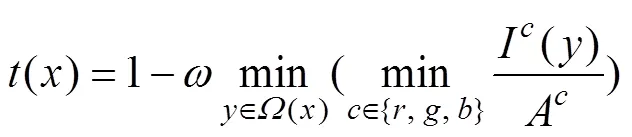
whereis a color channel ofandis a local patch centered at. The statistical observations state thatdark→0. Given an input image, suppose the ambient lightin Eq. (1) can be evaluated, the transmittance of the dark pixel in a local patch can be directly estimated from Eq. (1) as in (He, 2009)

whereis the control parameter.

With the assumption that the transmittance is constant in a local patch, the initial transmittance map can thus be obtained by applying Eq. (3) to each patch over the input image. Given that the formal DCP method is patch-based, the block effect is inevitable and the filter algorithm,., the guided filter or soft mating is needed to refine the final estimate.

and we have

whereis the control parameter.

To estimate the ambient lightA, we adopted the robust approach in feature detection of a sky region (Guo, 2014). Three distinctive features of the sky region are selected as follows: i) a bright minimal dark channel, ii) a flat intensity, and iii) an upper position. However, given that the observation of the sky light may be a mixture of the pure backscattered light and the sunlight, the estimate ofAmay be an overevaluated result. Therefore, a weighting coefficient onAwhose value is empirically determined, which is usually equal or smaller than a unit, needs to be imposed.

The DCP is based on a kind of statistics; it fails to output the correct estimates for pixels where the albedo of the objects is white or grayish because none of the RGB channels is dark. In such cases, the transmittance of those pixels by using the DCP algorithm is wrongly estimated. However, the DCP is valid for most of the pixels of a natural image; most pixels in the adjacent regions of the wrongly estimated pixels output the correct estimates of the transmittance. Given that the wrongly estimated pixels are within sparsely distributed regions, spatial depen- dencies of the well estimated and wrongly estimated pixels can give rise to the adjusted version of the transmittance map, which is formally characterized by the MRF model.

3 Estimation of the Transmittance Map Using the MRF Model

In general, the MRF model associates an image fieldwith the labeling of a variable seton the defined neigh- borhood. The labeling of the variable setcan thus be obtained by minimizing the cost function as follows:

The minimization of(?) can be interpreted as the MAP optimization, where1(?) represents the conditional probability and2(?) represents the priors that characterize the spatial dependencies of the neighborhood. Here, the input imagespecifies the dark channel image, and the variablespecifies the transmittance. By characterizing the cost function(?), we can obtain the refined estimate of the transmittance map.

3.1 Characterization of the MRF Model

As mentioned in Section 2, we obtain the pixel-based initial estimate of the transmittance by applying the DCP algorithm, which outputs the dark channel imagedarkIn the dark channel image, given thatdark→0, we havedark→A(1?), according to Eq. (1). Thus, the linear dependency of the dark channel image and the transmittance allows for the explicit characterization of the labeling of the transmittance by the observation of the input image. We define=1?and specify the MRF model on; the dark channel imagedarkis just an observation ofin the form

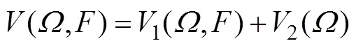
We then define a labeling of the variable, denoted asf; the observation of, denoted asfis evaluated from Eq. (7). Then, the cost function of Eq. (6) can be formulated as

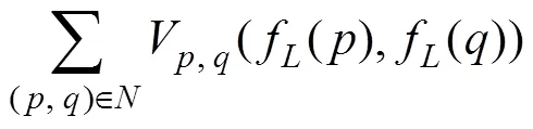
whereis the pixel on imagedark,is the neighbor of, andis the 8-connected neighborhood. In Eq. (8), the first termV(?) is the data function that indicates the cost or penalization of assigning a label to a pixel if it is too different from the observed data. The second termV, q(?) is a smoothing function that indicates the cost or penalty of assigning two neighboring pixels different labels if they are too close.

Usually, the conventional Gaussian probability model,.,V=(f()?f()), is used in the data function to describe the difference between the observation and the label. Such a model assumes that the error is just the random fluctuations in observations. Given the wrongly estimated transmittance here, however, it is not adopted to describe the systematic error caused by the invalid observation of the DCP method. Instead, we characterize the data function in the form

whereis the weighting parameter.

The curve described by Eq. (9) indicates that in case of correct estimates of the transmittance, the error of (f()?f())2is caused by the small noise of the observation so that the sharp changeVof at small errorsensures sufficient penalization to a small error. In case of wrong estimates of the transmittance, however, the error is large but the change ofVis slow, implying a relatively weak penalization or larger tolerance of such a systematic error. Therefore, the specification of the data function of Eq. (9), incorporated with the smoothing termV, q, increases the possibility of assigning the wrongly estimated pixel to the same label of its correctly estimated neighbors according to statistics.

The choice ofV, q(?) is a critical issue in the MRF model. While some typical models such as the Ising (Besag, 1986) and Potts (Tu and Zhu, 2002) models are available, the characterization of the coherence of neighboring pixels is usually domain-specific. For the dehazing problem, a trade-off exists between the smoothness of the transmittance at the same depth and the sharpness at the depth discontinuity. In the proposed method, the initial estimate of the transmittance map is pixel-based rather than patch-based, thus requiring sufficient smoothing to adjust the wrongly estimated transmittance of the regions neighboring those that are well estimated. Meanwhile, the uncertainties of pixel-based estimates due to image noise can be properly depressed. The number of labels is also relevant to the choice of the smoothing term. We characterize the smoothing term as follows:

where1is the weighting parameter.

The smooth function encodes the probability, whereby neighboring pixels should have a similar depth. However, edges usually occur with a large difference between f() andf(). Traditional smooth functions such as(f()?f())2and (f()?f()) may result in discontinuous edges, whereas our smooth function could perform better in edge preservation.

To minimize the cost function of Eq. (8), we apply the graph cut technique (Boykov, 2002; Delong, 2012) and employ the α-expansion algorithm to solve the graph cut problem with good computational performance.

3.2 Labeling the Transmittance Map with Clustering and Segmentation

Most dehazing algorithms assume that the depth map of the outdoor scene is smoothly varying over the whole image. However, the scene does not need to be continuous where the objects are grouped at different depths in the field of view, which means that the depth and the trans- mittance associated with the objects may be frequently distributed in discontinuity. Such a fact or prior suggests that we can reasonably cluster the transmittance map of the scene with a limited number of labels instead of the whole dynamic range of the gray level, which can effectively reduce the computational cost of Eq. (8).

Further investigations show that a large discontinuity of the scene depth,., in the appearance of the foreground and background of the image, may result in artifact problems at the discontinuity when the MRF model is applied to the whole image; the smoothing term in the MRF model cannot properly smooth the discontinuity of two segments that are spatially non-correlated. Therefore, we have to identify the foreground and background of the image before applying the MRF model. We apply the Otsu segmentation method to the initial transmittance map and apply the morphological filter to refine the results, as shown in the example of Fig.1. We then apply the MRF model to the segmented foreground and background se- parately without smoothing at the discontinuity of these two kinds of pixels.

To initialize the labels, we apply the-means clustering algorithm to cluster the transmittance map; the center of each cluster consists of the initial estimates of the labeling off. The number of clusters is manually preset the same as the labels.

The label initialization by clustering is implemented on the result of patch-based estimates of the transmittance map by using He’s method (He., 2009) rather than thepixel-based result because the pixel-based result may cause more variations among neighboring pixels than the patch- based result. The patch-based result can reduce the risk of assigning estimated neighboring transmittance to different clusters.

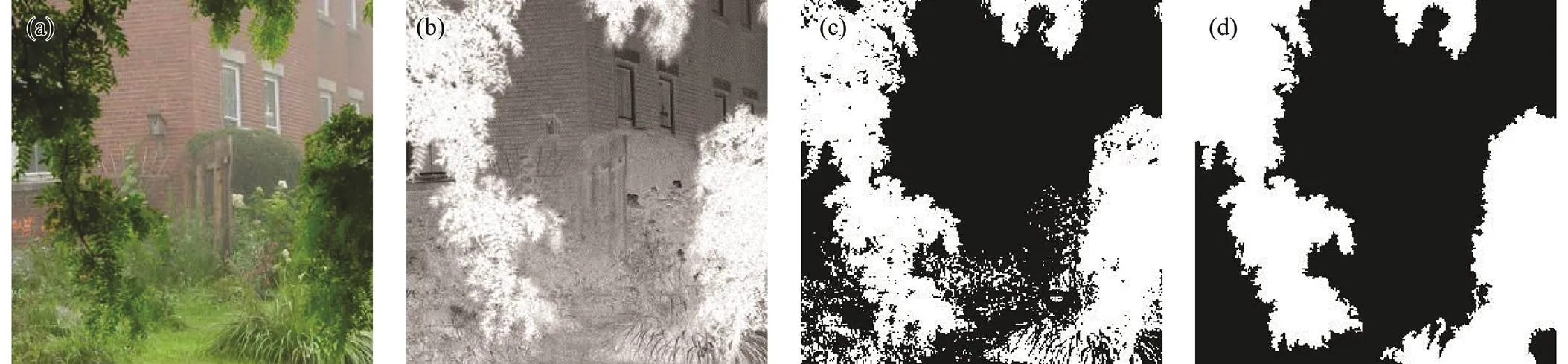
Fig.1 Segmentation of the transmittance map into the foreground and background. (a), Input image; (b), transmittance map using pixel-based DCP; (c), segmentation result; (d), refinement using morphological filter.

4 Experimental Results

We evaluated the proposed algorithm on terrestrial and underwater images. In our experiments, the number of labels in the MRF model is selected with=24,=0.2,1=10. Given that the estimation of the initial transmittance map is pixel-based rather than patch-based in the proposed method, the block effect is avoided; the transmittance map is smoothed by optimizing the smoothing term in the MRF model. Therefore, no extra filter stage, such as the guided filter, was employed to refine the transmittance map.

Fig.2 shows the results of the transmittance map obtained using the proposed method and that obtained by using He’s method (He, 2009). The patch size is selected as 15×15 in He’s method, which is also used for clustering in our method. Local white regions are present in the scene (within the red window in Fig.2(b)) where the DCP does not work so that the transmittance of those regions is underestimated by He’s method. The proposed method effectively adjusts the initial estimates and outputs the revised version of the transmittance map. To further evaluate the difference between both methods, we plot the curves of the transmittance along a line segment with respect to both methods, as shown in Fig.2(d). The de- hazed outputs using both methods are shown in Figs.2(e) and 2(f), respectively.

We compared the transmittance map obtained using the proposed method and that obtained using He’s method for terrestrial and underwater images. Figs.3–7 show the results.

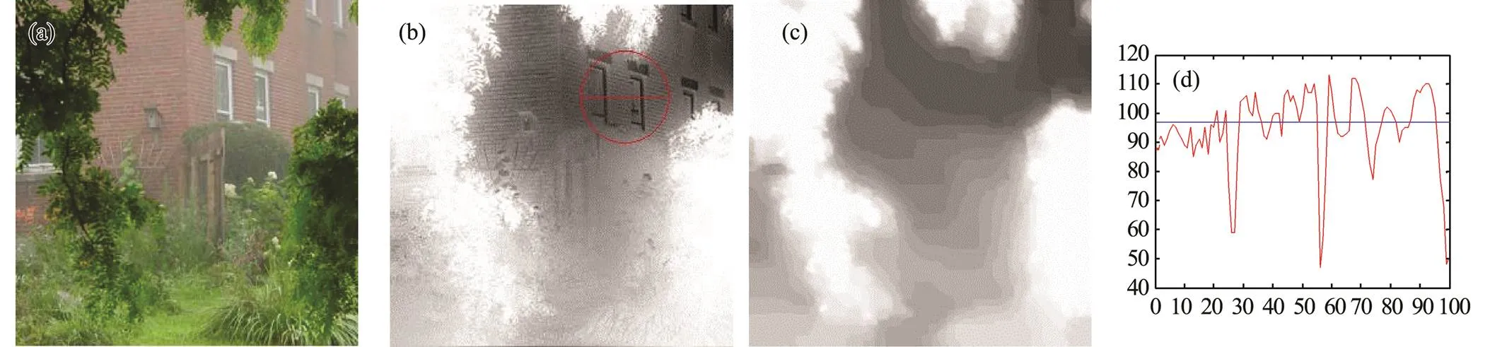
Fig.2 Image ‘house’. (a), Input image; (b), transmittance map by He’s method; (c), transmittance map by the proposed method; (d), comparison of the change of transmittance along the line segment as shown in (b), with respect to He’s method (red) and the proposed method (blue).

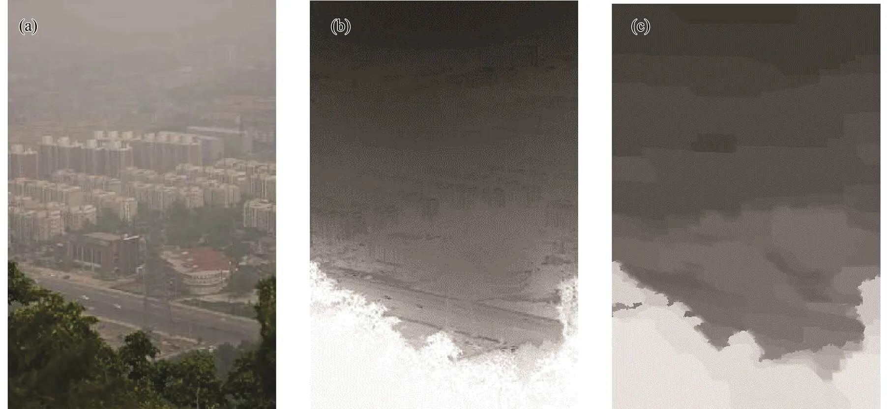
Fig.3 Image ‘city road’. (a), Input image; (b), transmittance map by He’s method; (c), transmittance map by the proposed method.

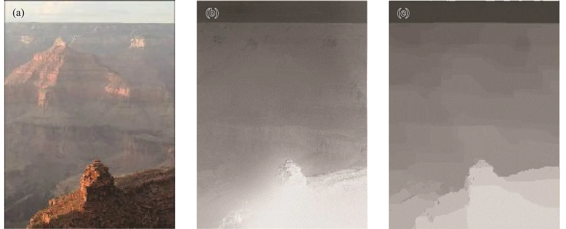
Fig.4 (a)–(c) are same as Fig.3, but (a) input image is ‘tsuchiyama’.

Fig.5 (a)–(c) are same as Fig.3, but (a) input image is ‘tree hills’. Note the difference of the transmittance maps on the local white house (marked in red).

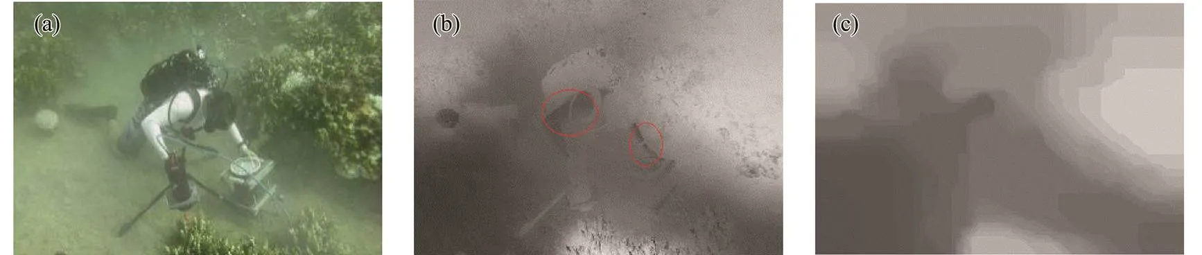
Fig.6 (a)–(c) are same as Fig.3, but (a) input image is ‘driver’. Note the difference of the transmittance maps on the local white house (marked in red).

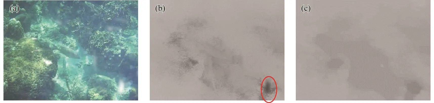
Fig.7 (a)–(c) are same as Fig.3, but (a) input image is ‘creek’. Note the difference of the transmittance maps on the local white house (marked in red).

We compared our proposed method with several other widely mentioned algorithms for terrestrial and underwater images. Figs.8–12 show a comparison of the results obtained by the methods of He (He, 2009), Tarel (Tarel and Hautiere, 2009), Meng (Meng, 2013), Zhu (Zhu, 2015), Kim (Kim, 2013), and the proposed method.

In our proposed method, although the transmittance is labeled with a limited number (64 in our experiments), neither block effects nor artifacts appear in the dehazing results; the outputs were properly refined by optimizing the MRF model, incorporated with the initialization of clustering and segmentation of the transmittance.

The proposed method takes about 22–30 seconds to pro- cess a 640×480 image on an Intel Core i5 4200M CPU and the memory consumption is approximately 1GB, while He’s method (using guide filter) takes about 10 seconds.

To evaluate the proposed method quantitatively, we apply an assessment metric dedicated to visibility restoration proposed in (Hautiere, 2008) to measure the contrast enhancement of the dehazed images in Figs.8– 12.

We first transform the color-level images into gray- level images and use the three indicators to compare two gray-level images: the input image and the fog removal image. The rate of edges that are newly visible after dehazing is evaluated and the results, denoted as the indicator, are given in Table 1.

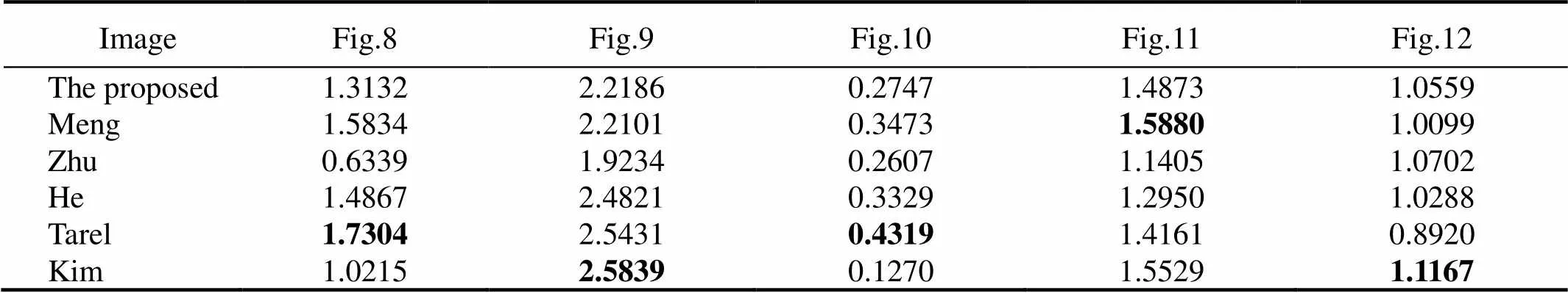
Table 1 Quality assessment by the indicator e

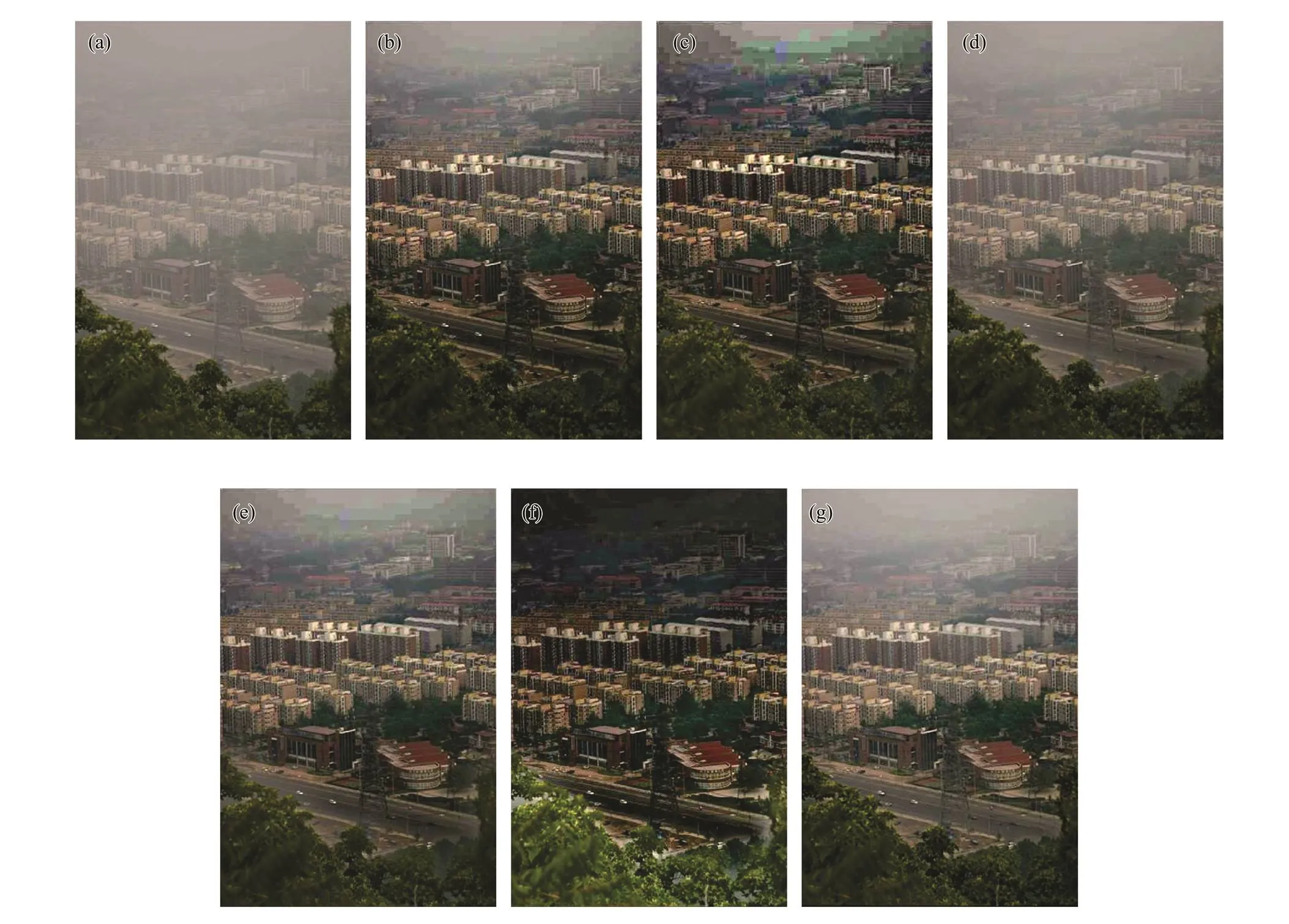
Fig.8 Image ‘city road’. (a), Input image. (b)–(g) are the dehazing result obtained by the proposed method and the methods used by Meng, Zhu, He, Tarel, and Kim.

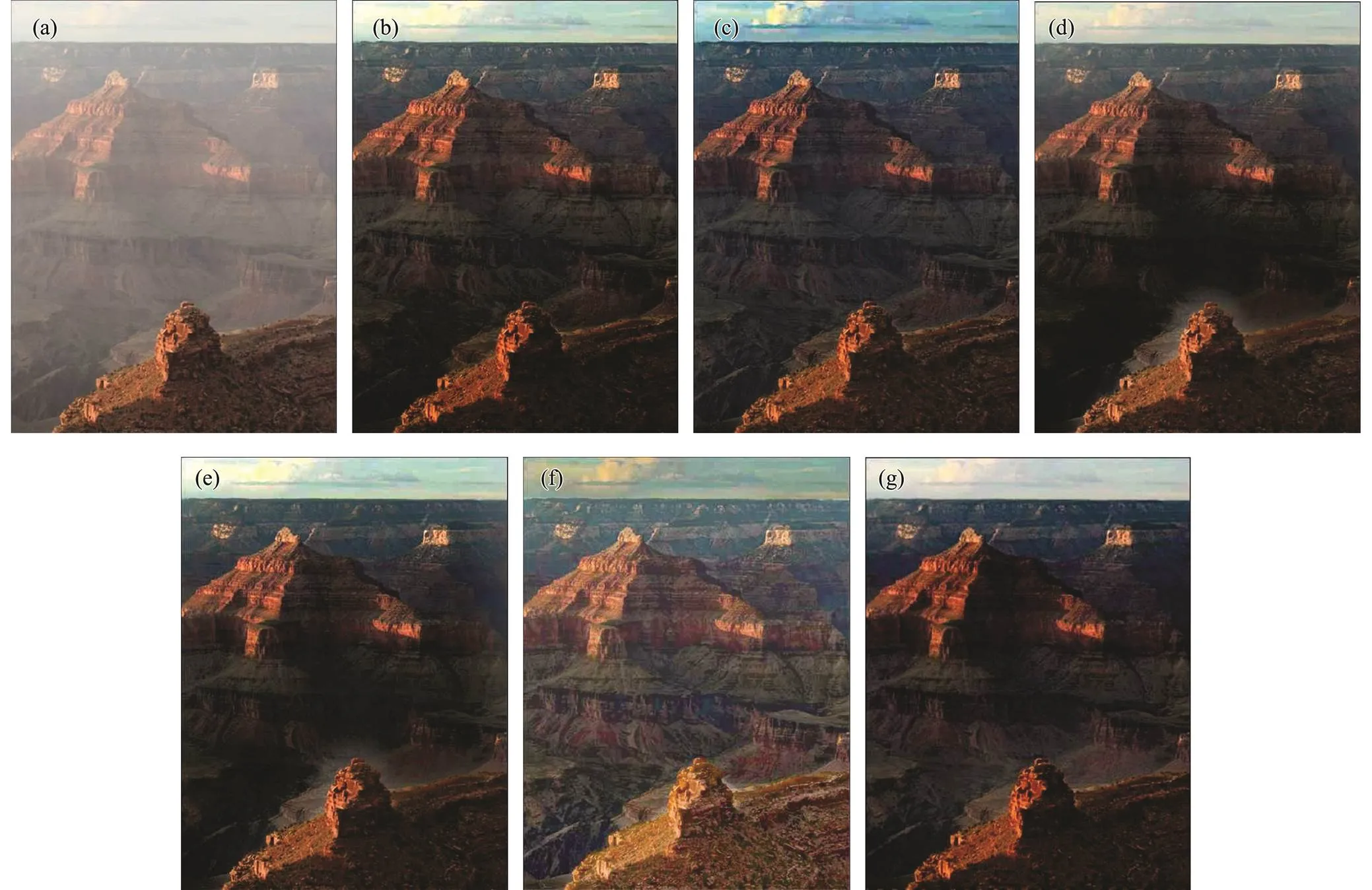
Fig.9 (a)–(g) are same as Fig.8, but (a) input image is ‘tsuchiyama’.

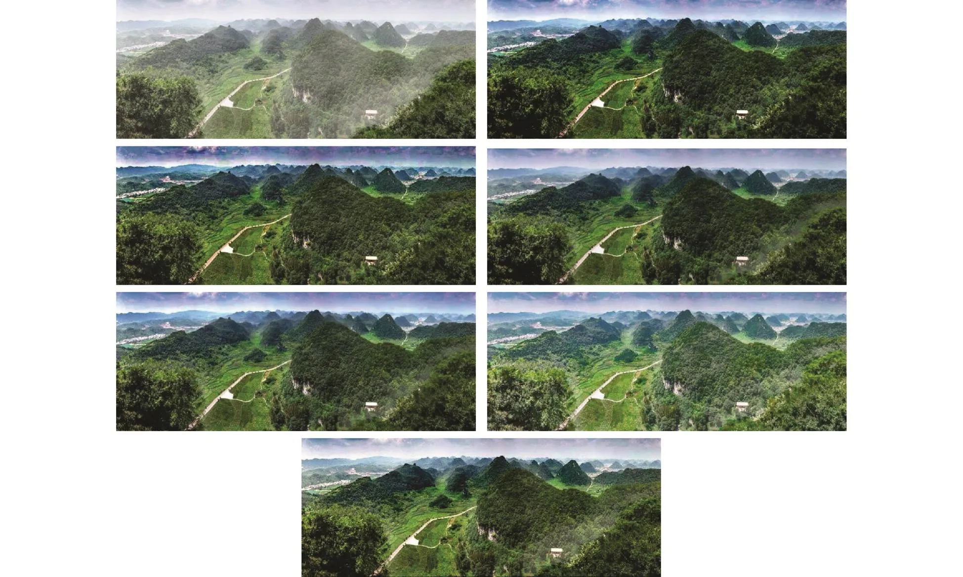
Fig.10 (a)–(g) are same as Fig.8, but (a) input image is ‘tree hills’.

Fig.12 (a)–(g) are same as Fig.8, but (a) input image is ‘creek’.

To assess the average visibility enhancement, the mean of the ratio of the gradient norms over these edges both before and after dehazing, denoted as the indicator, is evaluated, and the results are given in Table 2.

The percentage of pixelsthat become completely black or completely white after restoration is given in Table 3.

Each method aims to increase the contrast without losing visual information. Hence, according to paper (Hau- tiere, 2008), good results are always described by high values of e and I and low values of. Tables 1 to 3 show that Tarel’s algorithm generally performs better in all three indicators. However, the experiments show that the algorithms with more visible edges probably increase the contrast too much such that the fog removal images may have halos near some edges and the color seems unnatural. This finding confirms our observations regarding Figs.8 to 12.

Table 2 Quality assessment by the indicator r

Table 3 Quality assessment by the indicator σ

To better evaluate the proposed method, we choose three full-reference approaches (PSNR, MSE, and SSIM) based on synthesized images. First, we synthesize images for evaluation according to the ground truth images, and two ground truth images, for which the depth maps are known, were used to synthesize images. Figs.13–14 show a comparison of the results obtained by our method and He (He, 2009), Tarel (Tarel and Hautiere, 2009), Meng (Meng, 2013), Zhu (Zhu, 2015), and Kim (Kim, 2013).

The results in Table 4 show that the proposed method and Zhu’s method perform better than the other methods in most cases.

Fig.13 (a) Synthesized image; (b), ground truth image; (c)–(h) are the dehazing result obtained by the proposed method and the methods used by Meng, Zhu, He, Tarel, and Kim.

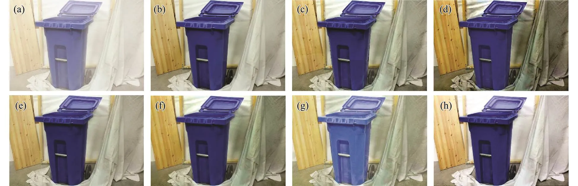
Fig.14 (a), Synthesized image; (b), ground truth image; (c)–(h) are the dehazing result obtained by the proposed method and the methods used by Meng, Zhu, He, Tarel, and Kim.

5 Conclusions

This paper proposes an algorithm by using the MRF model and the DCP for image dehazing. Given that the DCP is based on the statistics of natural images, it is invalid for local scenes where none of the RGB channels is dark, such as white or gray objects. Thus, the transmittance of the local scenes is wrongly estimated by using the DCP method even though an extra filter stage is applied to refine the transmittance map. The proposed method is used to adjust the wrongly estimated transmittance by characterizing the smoothing term in the MRF model, which utilizes the spatial dependencies among the neighboring pixels of the well estimated and wrongly es- timated transmittances. The data function and the smoothing function of the MRF model were designed specifically for this purpose. The experimental results show that the proposed method can effectively correct the wrongly estimated transmittance map. Moreover, given that the estimation of the initial transmittance map is pixel-based using the DCP, the block effect is avoided and the smoothing term in the MRF model can properly smooth the transmittance map so that further refinement by a dedicated filter is no longer required.

Table 4 Quality assessment by PSNR, MSE, and SSIM

The proposed algorithm assumes that the wrongly estimated pixels are located in sparsely distributed regions, while the DCP is valid for most of the regions of the scene. In case the wrongly estimated pixels are grouped in sufficiently large local regions, the proposed method would fail to work effectively. The number of labels and the initial clustering also affect the performances of the method. For most of the images in our experiments, labels of={32, 64} can result in good-performing outputs. Large numbers induce more computational cost with little refinement, while smaller ones induce block effects and degrade the local contrast of the output image.

Acknowledgement

This work was supported by the National Natural Science Foundation of China (No. 61571407).

Besag, J., 1986. On the statistical analysis of dirty pictures.,48 (3): 259-302.

Boykov, Y., Veksler, O., and Zabin, R., 2003. Fast approximate energy minimizationgraph cuts., 23 (11): 1222-1239.

Cataffa, L., and Tarel, J. P., 2011. Markov random field model for single image defogging..Gold Coast, USA,994-999.

Chiang, J. Y., and Chen, Y., 2012. Underwater image enhancement by wavelength compensation and dehazing., 21 (4): 1756-1769.

Delong, A., Osokin, A., Isack, H. N., and Boykov, Y., 2012. Fast approximate energy minimization with label costs., 96 (1): 1-27.

Drews Jr., P., Nascimento, E., Moraes, F., Botelho, S., and Cam-pos, M., 2013. Transmission estimation in underwater single images.. Sydney, Australia, 825-830.

Fattal, R., 2008. Single image dehazing., 27 (3): 1-9.

Guo, F., Tang, J., and Peng, H., 2014. A Markov random field model for the restoration of foggy images., 11 (1): 1-14.

Hautiere, N., Tarel, J. P., Aubert, D., and Dumont, E., 2008.Blind contrast enhancement assessment by gradient ratioing at visible edges., 27 (2): 87-95.

He, K., Sun, J., and Tang, X., 2009. Single image haze removal using dark channel prior., 33 (12): 2341-2353.

Hitam, M. S., Yussof, W. N. J. H. W., Awalludin, E. A., and Bachok, Z., 2013. Mixture contrast limited adaptive histogram equalization for underwater image enhancement..Sousse, Tunisia, 1-5.

Iqbal, K., Salam, R. A., Osman, A., and Talib, A. Z., 2007. Underwater image enhancement using an integrated color model.,34(2): 529-534.

Kim, J., Jang, W., Sim, J., and Kim, C., 2013.Optimized contrast enhancement for real-time image and video dehazing., 24 (3): 410-425.

Kratz, L., and Nishino, K., 2009. Factorizing scene albedo and depth from a single foggy image.. Kyoto, Japan,ICCV. 2009. 5459382.

Meng, G., Wang, Y., Duan, J., Xiang, S., and Pan, C.,2013. Efficient image dehazing with boundary constraint and contextual regularization..Sydney, NSW, Australia, 2013.82.

Narasimhan, S. G., and Nayar, S. K., 2002. Vision and the atmosphere., 48 (3): 233-254.

Nishino, K., Kratz, L., and Lmbardi, S., 2012. Bayesian defogging., 98 (3): 263- 278.

Tan, R. T., 2002. Vision and the atmosphere., 48 (3): 233-254.

Tarel, J. P., and Hautiere, N., 2010. Fast visibility restoration from a single color or gray level image.. Kyoto, Japan, 2201-2208.

Treibitz, T., and Schechner, Y. Y., 2009.Active polarization de- scattering., 31 (3): 385-399.

Tu, Z., and Zhu, S. C., 2002. Fast approximate energy minimizationgraph cuts., 24 (5): 657-673.

Wang, Y. K., Fan, C. T., and Chang, C. W., 2013. Accurate depth estimation for image defogging using Markov random field..Singapore, 87681Q, 1-5.

Wong, S. L., Yu, Y. P., Ho, A. J., and Paramesran, R., 2014. Comparative analysis of underwater image enhancement me- thods in different color spaces.. Kuching, Malaysia, 34-38.

Zhu, Q., Mai, J., and Shao, L., 2015. A fast single image haze removal algorithm using color attenuation prior., 24(11): 3522-3533.

# These authors contributed equally to this work.

. E-mail: gywang@ouc.edu.cn

September 12, 2018;

May 29, 2019;

August18, 2019

(Edited by Chen Wenwen)