A modified method of discontinuity trace mapping using threedimensional point clouds of rock mass surfaces

Keshen Zhng, Wei Wu,*, Hehu Zhu, Linyng Zhng, Xiojun Li, Hong Zhng

a Department of Geotechnical Engineering, Tongji University, Shanghai, 200092, China

b Department of Civil Engineering and Engineering Mechanics, University of Arizona, Tucson, AZ, 85721, USA

c Department of Hydraulic Engineering, Tongji University, Shanghai, 200092, China

Abstract This paper presents an automated method for discontinuity trace mapping using three-dimensional point clouds of rock mass surfaces. Specifically, the method consists of five steps: (1) detection of trace feature points by normal tensor voting theory,(2)contraction of trace feature points,(3)connection of trace feature points, (4) linearization of trace segments, and (5) connection of trace segments. A sensitivity analysis was then conducted to identify the optimal parameters of the proposed method.Three field cases, a natural rock mass outcrop and two excavated rock tunnel surfaces, were analyzed using the proposed method to evaluate its validity and efficiency. The results show that the proposed method is more efficient and accurate than the traditional trace mapping method, and the efficiency enhancement is more robust as the number of feature points increases.

2020 Institute of Rock and Soil Mechanics, Chinese Academy of Sciences. Production and hosting by Elsevier B.V. This is an open access article under the CC BY-NC-ND license (http://creativecommons.org/licenses/by-nc-nd/4.0/).

Keywords:Rock mass Discontinuity Three-dimensional point clouds Trace mapping

1. Introduction

Discontinuity trace mapping plays an important role in characterizing rock masses. Discontinuities have a significant effect on the strength,deformability and permeability of rock masses(Zhang and Einstein, 1998; Zhang, 2017), which are often characterized based on the information from discontinuity trace mapping(Mauldon,1998;Zhang and Einstein,2000;Li et al.,2014;Zhu et al.,2014). Discontinuity trace is one of the seven major parameters suggested by the International Society for Rock Mechanics (ISRM,1978) to quantitatively describe rock discontinuities. The information of discontinuity traces is obtained traditionally through conducting geotechnical field survey with a tape and a geological compass(Franklin et al.,1988).However,the traditional field survey is time-consuming in conjunction with safety concerns,and has its biases and cannot be easily accomplished correctly or completely(Crosta,1997;Priest and Hudson,1981;Kulatilake et al.,1993;V?ge et al., 2013). Recently, emerging non-contact methods, including photogrammetry and light detection and ranging (LIDAR) technology, have been introduced to obtain discontinuity information via images and three-dimensional (3D) point clouds of rock mass surfaces.These technologies can greatly improve the efficiency of in situ data collection due to convenient operation.The uniform data format and mapping algorithm also make it possible to extract more accurate, objective and credible information of discontinuities.

The two-dimensional(2D)image method of discontinuity trace mapping is based on the gray-level variation and distribution of pixels(Crosta,1997;Franklin et al.,1988;Reid and Harrison,2000;Hadjigeorgiou et al., 2003). However, the method shows strong dependence on image quality, which is easily influenced by dust,illumination,noise and production constraints,and often generates meaningless segments or excessive fragmentation (Lemy and Hadjigeorgiou, 2003; Ferrero et al., 2009). In addition, the images produced by uncalibrated cameras suffer from lens distortion and projective distortion which are hard to rectify (Li et al., 2016).

Recently, many researchers have studied discontinuity trace mapping using 3D point clouds of rock mass surfaces(Roncella and Remondino, 2005; Gigli and Casagli, 2011; Li et al., 2016; Ge et al.,2018; Guo et al., 2018). The 3D point clouds of rock mass surfaces can be obtained using either LIDAR or photogrammetry(Kraus and Pfeifer,1998;Chandler,1999; Lane et al., 2000). Although LIDAR is more convenient than photogrammetry in acquiring point cloud directly, it is difficult to cover all relevant viewing directions and achieve good registration of scans and sufficient resolution for steep terrains or surfaces with vegetation. The photogrammetry is in principle more flexible because the image scale and viewing direction can be more easily adapted to the need (Roncella and Remondino, 2005). Two types of methods have been used to detect discontinuity traces from 3D point clouds of rock mass surfaces.The first one considers a discontinuity trace as an intersection line between two adjacent fitting planes of rock mass surfaces.Gigli and Casagli,(2011)presented a 3D trace recognition method which projects 2D traces obtained from image processing on the intersections of corresponding 3D discontinuity fitting planes.However, the effectiveness of trace mapping is heavily dependent on the accuracy of both the 2D traces on images and the 3D fitting planes,which results in the difficulty to precisely recognize the 3D spatial locations of traces. The second type detects discontinuity traces from vertices which constitute the rock mass surface and are located around the real traces. In Umili et al. (2013)’s method, the feature vertices consisting of the traces were first recognized using principal curvature values, and then the traces were expressed as straight lines after connection and segmentation. Similarly, in Li et al. (2016)’s method, the feature vertices were recognized by the normal tensor voting (NTV) theory (Page et al., 2002) and the traces were detected based on a growth algorithm.In the method of Ge et al. (2018), 3D point clouds data were first converted to grid data, and then the traces were detected using a modified region growing (MRG) algorithm.

Currently,the second method based on feature vertices is more widely used to detect discontinuity traces from the 3D point clouds model (Umili et al., 2013; Li et al., 2016; Zhu et al., 2016; Ge et al.,2018). However, since each of the feature vertices for a trace needs to be calculated, judged and selected, the process is very time-consuming. In addition, the intersection of multiple natural discontinuities with the rock surface and the damage due to construction blasting and disturbance may separate a natural discontinuity trace into trivial pieces, making it more difficult to detect traces.Therefore,the aim of this paper is to improve the efficiency and accuracy of discontinuity trace mapping from 3D point clouds of rock mass surfaces by proposing an automated mapping approach.

2. Methodology

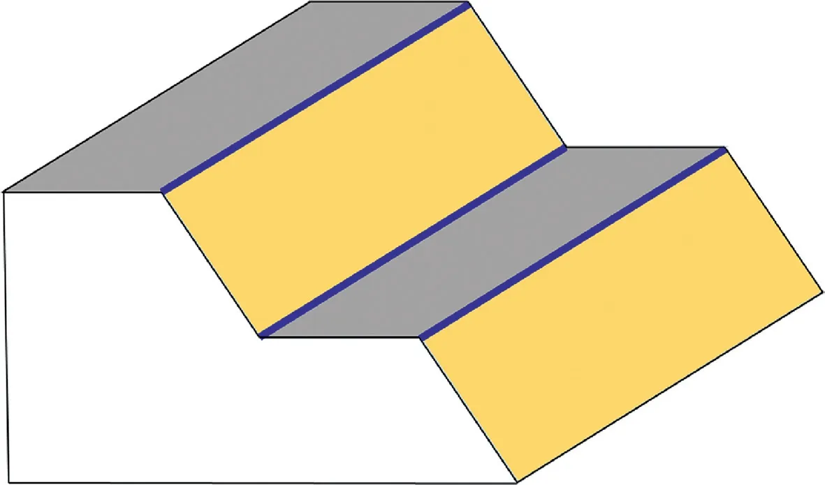
Fig. 1. Sketch figure of traces. This figure shows a conceptual model of a rock mass body.Gray plane and yellow plane represent two different sets of discontinuity planes,and the traces are three blue intersection lines of the two adjacent discontinuity planes.

Rock mass discontinuities include joints, bedding planes,faults, and other types of fracture planes (Kemeny and Post,2003). In this paper, a trace is defined as the intersection line of two adjacent discontinuity planes which belong to different sets (Fig.1).

The proposed automated method for discontinuity trace mapping includes five steps (Fig. 2):

(1) Identification of trace feature points with mesh vertices around a trace;

(2) Contraction of trace feature points together on their point cloud skeleton;

(3) Connection of trace feature points belonging to the same trace;

(4) Linearization of trace segments parted into linearized segments; and

(5) Connection of trace segments belonging to the same trace.

In the above phases,step(1)is the same as proposed by Li et al.(2016),step(2)is based on the theory proposed by Cao et al.(2010)and some modifications are made, and steps (3)e(5) are the improvements proposed in this paper.

Before applying the 5-step procedure, the 3D point clouds data need to be preprocessed to consider the disturbances and errors due to various factors such as vegetation, fragmentation,and dust (Slob et al., 2007). The preprocessing includes: resampling the point clouds using a minimum distance of 3 cm to reserve the rock mass geometry features, performing denoising using the moving least squares method (Alexa et al., 2003) to reduce noise, and acquiring a 3D surface model of the rock mass using the Delaunay triangulation algorithm (Li et al., 2016) and Halcon (MVTec Software GmbH, 2012). As a result of the preprocessing,triangular meshes of the 3D point clouds of rock mass surface are obtained.

2.1. Trace feature point detection

2.1.1. Normal tensor voting (NTV) method

Traces on triangulated meshes refer to as the skeleton of feature points composed of mesh vertices on edges and corners.Edges can be detected by surface normal variation within a neighborhood because the surface normal has an abrupt change across edges(Sun et al.,2002).Normal voting scheme,which is extended from tensor voting, can be performed to achieve robust detection. The voting scheme can be simply regarded as the eigenvalue analysis of a set of surface normals (Medioni et al., 2000). The NTV method can recognize sharp features and show robustness to noisy data.

Given a triangulated mesh is denoted byis the set of vertices, E is the set of edges andis the set of faces. Each vertexis represented using Cartesian coordinates, denoted byThe NTV of a vertex v is defined as

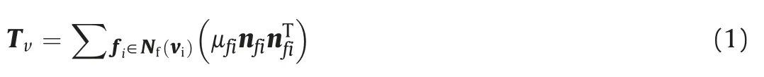
Fig. 2. Procedure for discontinuity trace mapping.

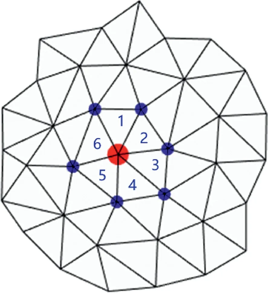
Fig.3. An example of one-ring neighbor points and Nfvi.Red point represents point vi, blue points are one-ring neighbor points of vi, and blue numbers are the corresponding one-ring neighbor face indices of vi. Therefore, Nfvi {1, 2, 3, 4, 5, 6}.

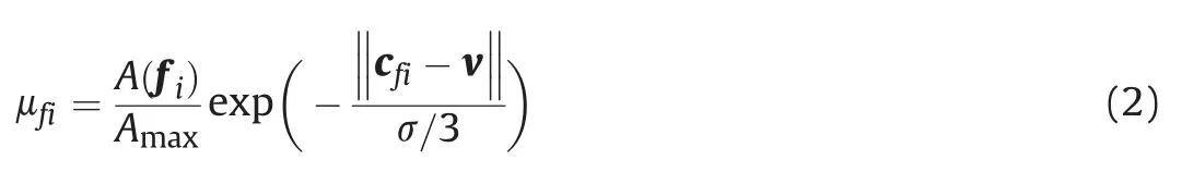
whereAfiis the area of triangle fi,Amaxis the maximum area ofAfi,cfiis the barycenter of triangle fi,andis the edge length of a cube that defines the neighbor space of each vertex.

In Eq. (1), Tvis a symmetric positive semi-definite matrix and can be represented as

According to the eigenvalues (Kim et al., 2009), vertices can be classified into three types: face type, sharp edge type, and corner type. The classification rules are as follows:

Feature points consist of both sharp edge type vertices and corner type vertices.

2.1.2. Detecting feature points

There are two thresholds, a and, defined to control the recognition accuracy of corner type and edge type points,respectively. Threshold value a should be large enough to avoid extracting over many false corners. Threshold valueis a finetuning coefficient around a value to find a tradeoff between detecting weak features and an extra number of noisy points(Wang et al., 2012). The definition of a anddepends on visual evaluation of the number of recognized edge type and corner type vertices (Li et al., 2016).

2.2. Trace feature point contraction

This step is based on the idea that traces are regarded as curve skeletons through adjacent feature points.Curve skeletons of point clouds can be extracted via a Laplacian-based contraction algorithm (Cao et al., 2010). The contraction algorithm can aggregate feature points on their skeletons using local Delaunay triangulation and topological thinning. Therefore, locations of 3D traces are obtained.

2.2.1. Trace feature point grouping

To reduce the mutual interference of contraction of different traces, feature points are grouped as follows: If viand vjare two vertices of the same triangulated mesh,then they are divided in one group.

2.2.2. Feature point contraction

Each group of the feature points is contracted as follows.

Given that a group of feature point isthe corresponding contracted set of point Vis obtained by solving the following system:

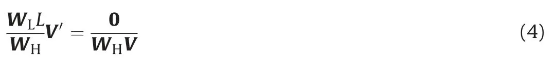
where WLand WHare the diagonal matrices that balance the contraction and attraction constraints, respectively (Au et al.,2008).

Eq. (4) is solved by the least-squares method, which is equivalent to minimizing the following quadratic energyEq(Sorkine and Cohen-Or, 2004):

where L is thenncurvature-flow Laplace operator with elements computed by Eq. (6). Because that the point clouds skeleton generated by one iteration of Eq. (4) is linear enough for trace mapping and time-saving, both WLand WHare defined as unit diagonal matrices in this step.

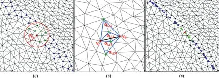
Fig. 4. Trace feature point contraction algorithm: (a) Positions of feature points before contraction (red circle represents the contraction scope, green points are the contraction neighbors of the red point,and the other feature points are plotted in blue);(b)Computation of i;j;and(c)Result of contraction(the positions of feature points before contraction are plotted in black).

Fig.5. Trace feature point connection algorithm:(a)Trace feature points before connection;(b)The criterion of trace feature point connection(the start point of the trace segment is plotted in the pink circle,the points added during connection are plotted in green,red points are the connection neighbors of the end point which is plotted in the green circle,and the 1/3 point v1=3 of the segment is plotted in black circle); and (c) Trace feature points after connection.

Fig.6. Trace segment linearization algorithm:(a)The trace segment before linearization;and(b)The result of the segment linearization in(a)and each color represents a linearized trace segment.

(1) Perform 3D Delaunay triangulation on all feature points V,and edge set E is obtained;

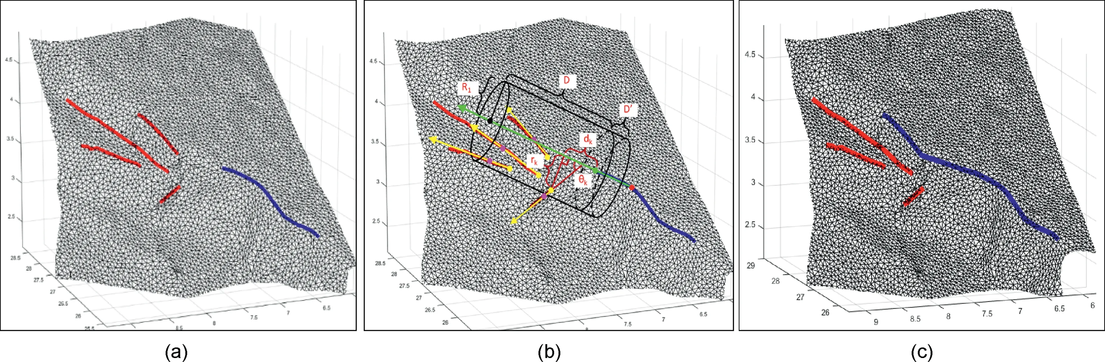
Fig.7. The trace segment connection algorithm:(a)The segments before connection(the blue segment is the one needed to be connected and the red segments are the ones that have not been connected); In (b), endpoint needed to connected is plotted in green, endpoints which have not been connected are plotted in yellow, and pink and red points represent the 1/3 points of their belonging trace segments; (c) The connection result of (a), which is the stretched blue segment.

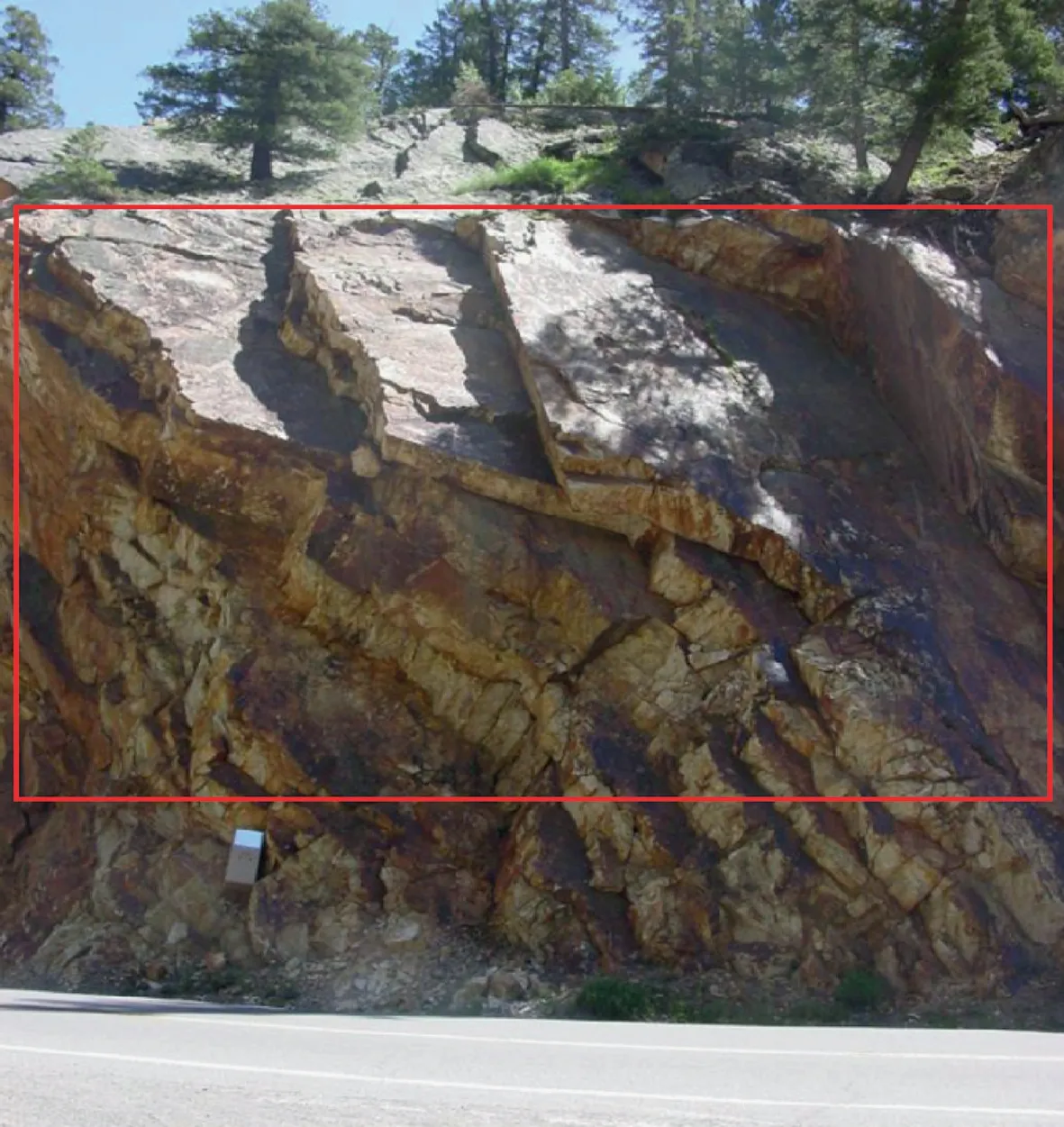
Fig.8. Real road cut slope analyzed in case study A.Image from Rockbench repository.Analyzed region is in the red frame.

(2) Calculate the distance between each feature point and its Delaunay neighbors;

(3) Define a contraction radiusR0(2.5 times the average edge length of triangular mesh,in Section 3.3),as shown in Fig.4a;and

(4) If the distance between a feature point and its Delaunay neighbor exceedsR0, then delete the neighbor point.Through iteration, the remaining Delaunay neighbors of a feature point are defined as contraction neighbors.

Through solving Eq. (4) once, viand its contraction neighbors can aggregate on their skeleton, as shown in Fig. 4c.

2.3. Trace feature point connection

The above procedures generate contracted feature points which aggregate on their point skeletons. This step is connecting the points to generate trace segments. Connection neighbors of contracted feature points are defined as Delaunay neighbors within connection radius.Because the contraction can enlarge intervals of the feature points that belong to the same trace segment,connection radius is defined larger than contraction radius, which is 3 times the average edge length of triangular mesh by data test.

Connection starts with a randomly selected point(pink point in Fig.5a)and chooses the nearest points of its connection neighbors as the possibly next point of the trace segment.

As shown in Fig.5b,given that the start point vsof the segment is in the pink circle,the end point veis in the green circle,the onethird point of the segment v1=3is in the black circle and the link point vpis possibly in the red circle. The connection rules are defined to control the connection direction as follows:

If vpsatisfies the connection conditions,it will be selected as the new end point(green point in Fig.5c);otherwise,the nearest point of the remaining connection neighbors of end point will be judged.The connection will end if none point of the remaining connection neighbors satisfies the connection conditions.

2.4. Trace segment linearization

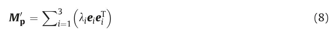
Because the algorithm of feature point connection in Section 2.3 might falsely connect feature points of different traces(Fig.6a),this step performs linear partition on trace segments to generate linearized segments which are composed only of the feature points of same traces.The method we used for trace segment linearization is called principal component analysis(PCA).Given a set of point VPCA analysis starts from calculating the covariance matrix:

wherenis the number of points,andc0is the centroid coordinate of the point clouds.Because the matrix Mpis symmetric and positive,it can be decomposed by eigenvalue as

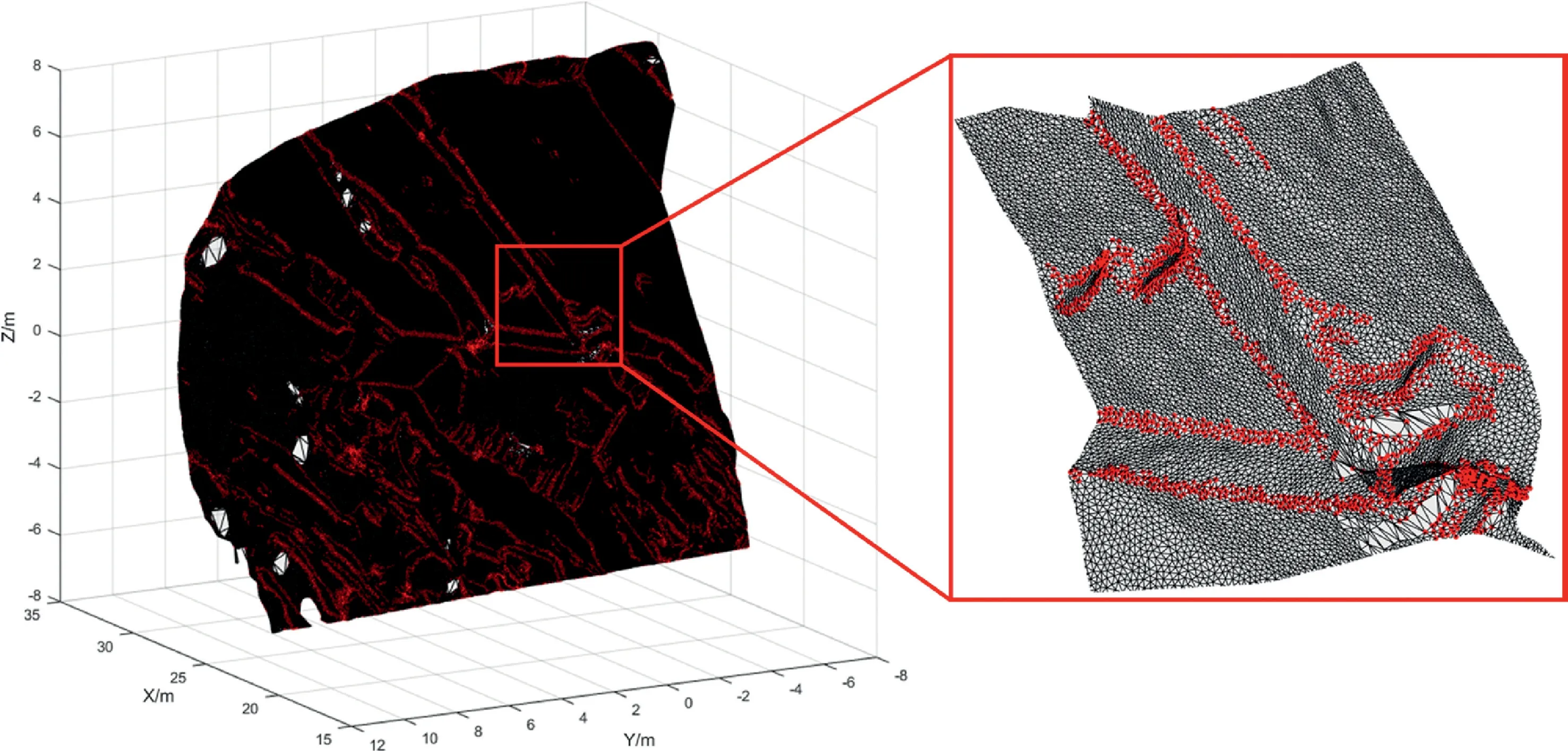
Fig. 9. Trace feature points. The triangular meshes are plotted in black.

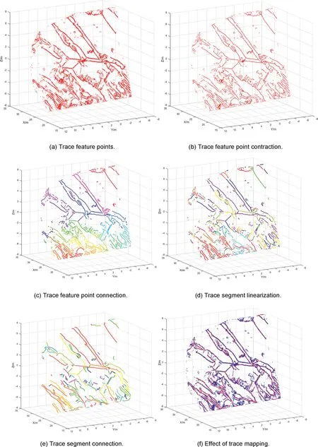
Fig.10. Trace mapping of case A.(aee)shows the trace mapping procedures of case A.Each color represents a trace.In(f),the blue segments are detected traces and the red points are feature points detected by NTV.

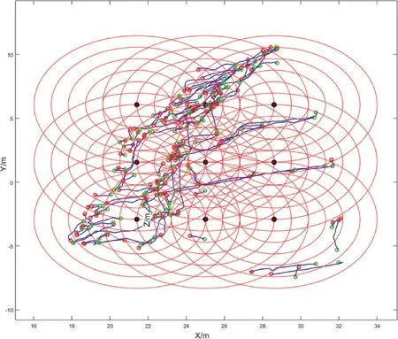
Fig.11. Trace projection of case A on the sampled plane of circular window method.

For each segment,the procedures of linearization are as follows:

(1) Computeuusing PCA algorithm;

(2) Ifuis smaller than linearization thresholdU, the trace segment is divided into two small segments containing same number of feature points; and

(3) For each divided segment, perform Steps (1) and (2) iteratively until all theuvalues of divided segments are greater than or equal toU, as shown in Fig. 6b.

2.5. Trace segment connection

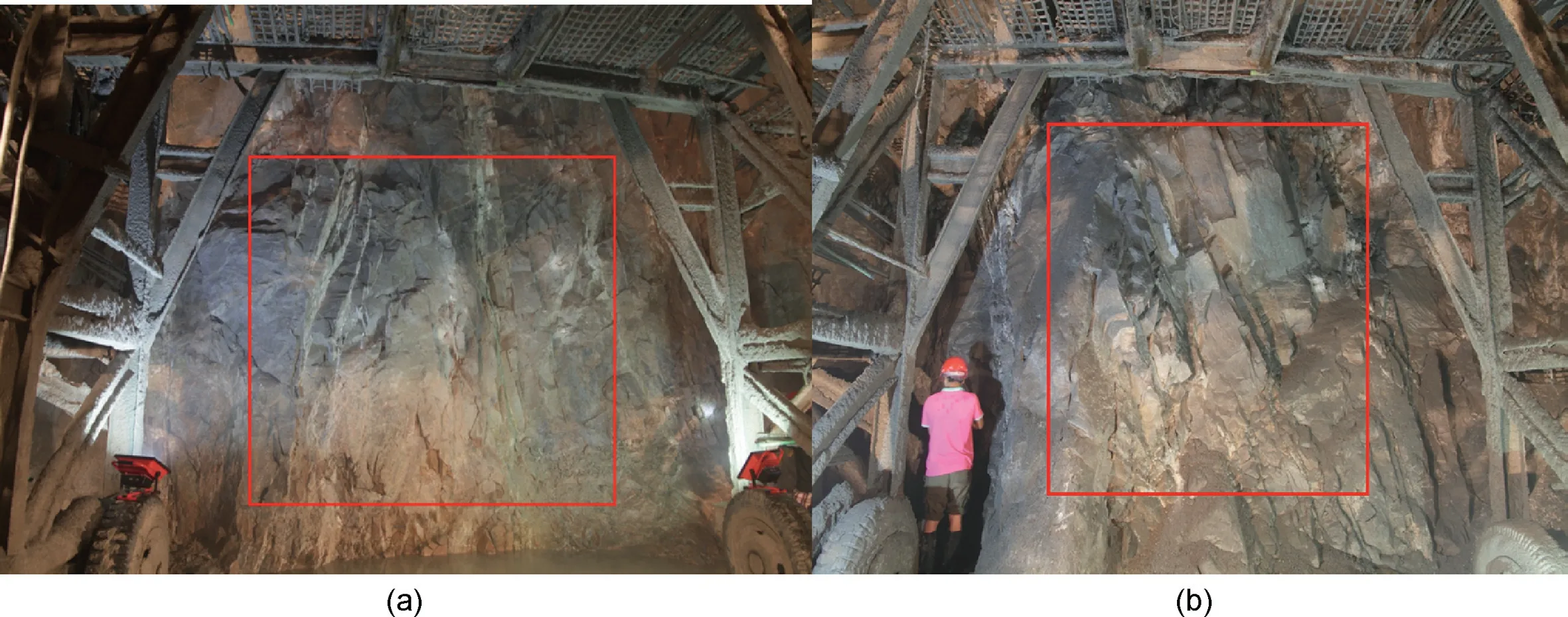
Fig.12. Tunnel excavation faces of case B.(a)shows the excavation face in ZK21 t 697.9 mileages and(b)shows the excavation face in ZK21 t 672.3 mileages.Analyzed region is in the red frame.

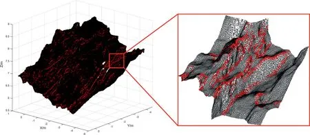
Fig.13. Trace feature points of case B(a). The triangular meshes are plotted in black.

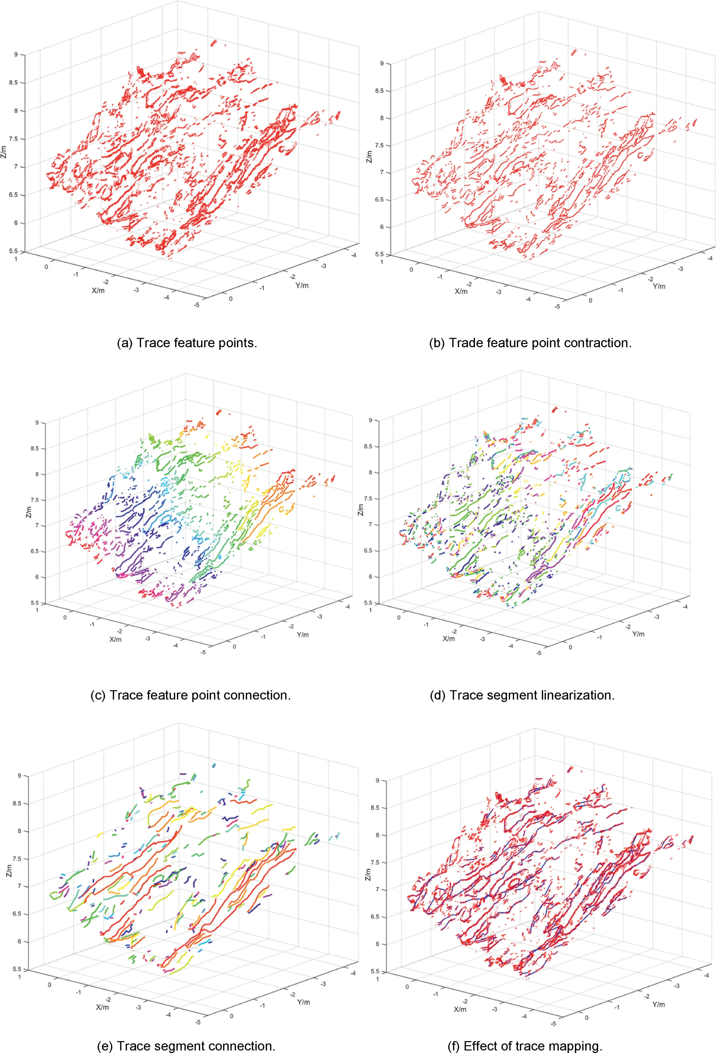
Fig.14. Trace mapping of case B(a).(aee)shows the trace mapping procedures of case B(a).Each color represents a trace.In(f),the blue segments are detected traces and the red points are feature points detected by NTV.

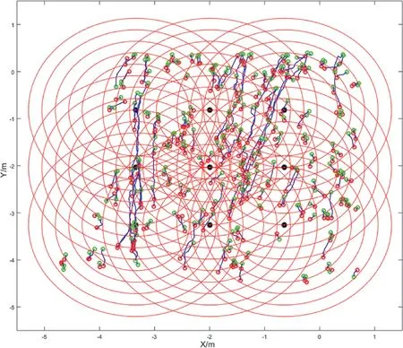
Fig.15. Trace projection of case B(a)on the sampled plane of circular window method.

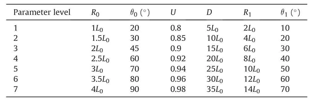
Table 1Threshold parameter level. Parameter L0 denotes the average edge length of triangular mesh.

Through the above analyses, we obtained discrete and linearized trace segments. In this section, the trace segments were connected to form continuous traces. Because that short linearized segments are affected more easily by noisy segments, the connection algorithm gives the long linearized trace segments the priority to be connected.As shown in Fig.7a,given the blue segment needs to be connected and the four red segments are the ones that have not been connected.As shown in Fig.7b,point vgthat needs to be connected is plotted in green, and possible connect points vyare plotted in yellow. Both vpand vrare one third points of corresponding segments and are plotted in pink and red, respectively.

The connection rules are defined as follows:

(2) Radial distanceis smaller than thresholdR1to control the radial extension;

(4) Given that the set S is composed of the segments which satisfy the above three conditions,the segment which should be connected is the one in S that has the minimum radial distancermin.

The segment withrminis selected to be the next connect segment because it is the nearest one to the extension cord of the under connect segment(as the blue segment shown in Fig.7a)and reflects the extension trend of trace most. Fig. 7c shows the connection result of Fig. 7a.

In the algorithm, the longest segment is connected first and the connection continues until none of the other segments satisfies the connection rules, and the longest segment of the remaining ones that have not been connected is the next to be connected. The algorithm proceeds until all segments are longer than thresholdL0(5 times the average edge length of triangular mesh by data test)connected.

3. Applications

3.1. Case A

3.1.1. Data description

The point cloud data of this case study were obtained from an available Rockbench repository(Lato et al.,2013).The natural rock mass outcrop of a road cut slope is located in Ouray,Colorado,USA.The scanning was carried out by an Optech Ilris3D scanner and obtained 1,515,722 points with the resolution of about 2 cm. The rock mass of this case is shown in Fig. 8 and the region under analysis is in the red frame.

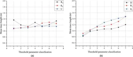
Fig.16. Mean trace length with different threshold parameter levels.

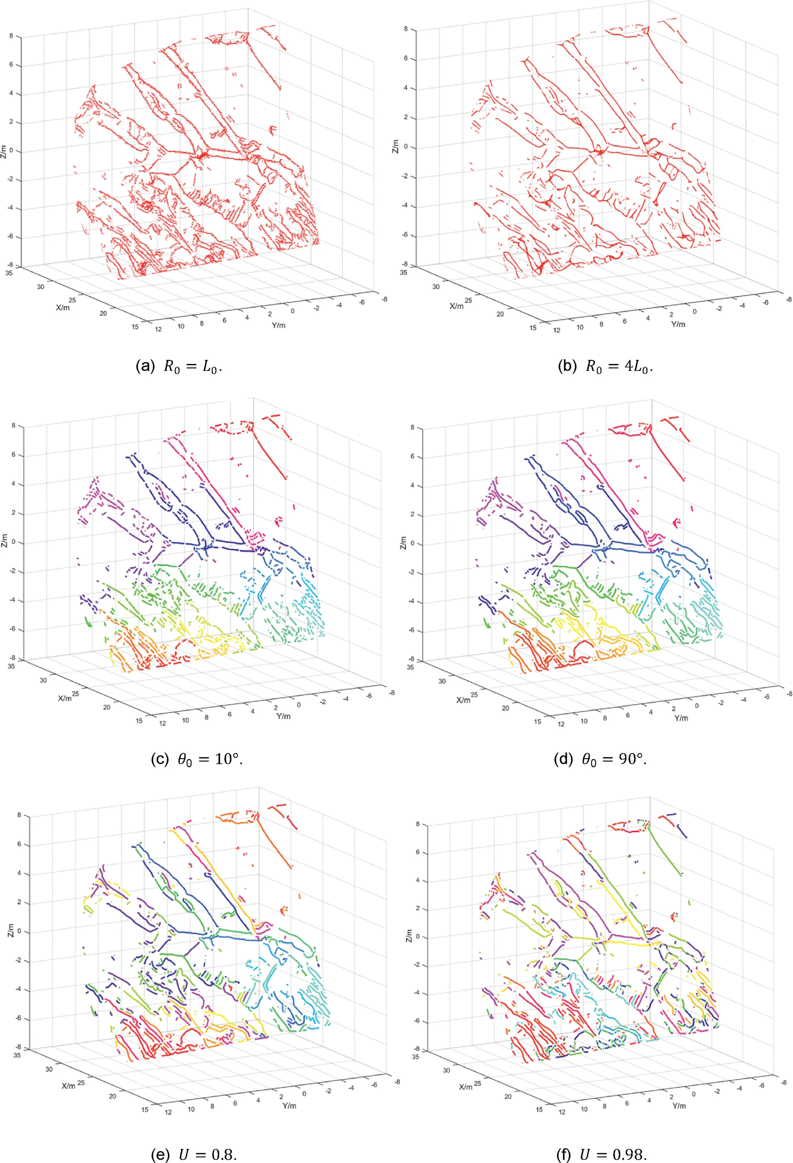
Fig.17. Trace mapping effect under different threshold parameters of R0;0 and U. Each color represents a trace.

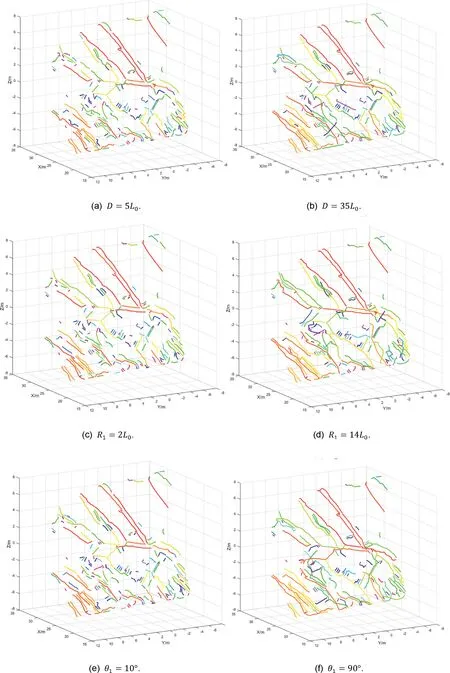
Fig.18. Trace mapping effect under different threshold parameters of D, R1 and 1. Each color represents a trace.

3.1.2. Trace mapping procedure

The feature points detected by NTV are shown in Fig.9.For clear observation,feature points without triangular meshes are shown in Fig.10a. Fig.10bee shows each step of the proposed method and Fig.10f shows both the feature points and the detected traces.

3.1.3. Mean trace length calculation

The mean trace length is calculated through the circular window sampling method (Zhang and Einstein, 1998) with an automated trace sampling procedure (Umili et al., 2013). Firstly, the detected traces were projected orthogonally on the sampling plane (XeYplane). Then, the centers of nine circular windows with five different radii were placed symmetrically on the sampled region.The radii are 10%, 15%, 20%, 25%, 30%, and 40% of the short edge length of sampled region. The mean trace length is calculated by(Umili et al., 2013):

whererdenotes the radius of circular window,mdenotes the number of traces with endpoints inside the circular window,andntdenotes the number of intersections which are between traces and the bounding circular scanline.Fig.11 shows the sampled plane of circular window method in case A.

3.2. Case B

3.2.1. Data description

The data of this case were obtained from two excavation faces of a highway rock tunnel in Yuexi County, Anhui Province, China (Li et al., 2016). The tunnel was 7.548 km long and was excavated using drill-and-blast method. The point cloud was obtained using overlapping photographs (Roncella and Remondino, 2005;Haneberg, 2008; Sturzenegger and Stead, 2009) to create 3D surfaces. Fig. 12 shows the excavation face and the 3D point clouds reconstruction region under analysis is in the red frame.

3.2.2. Trace mapping of case B(a)

The feature points detected by NTV are shown in Fig. 13. For clear observation, feature points without triangular meshes are shown in Fig. 14a. Fig. 14bee shows each step of the proposed method and Fig.14f shows both the feature points and the detected traces.

3.2.3. Mean trace length calculation

The method of mean trace length calculation was the same as that depicted in case A (Section 3.1.3). Fig.15 shows the sampled plane of circular window method.

3.3. Sensitivity analysis and calibration

Threshold contraction radiusR0, threshold angle0, linearization thresholdU,threshold distanceD,threshold distanceR1,and threshold angle1are important parameters for the proposed method for discontinuity trace mapping. Therefore, the sensitivity analysis will be performed on these parameters by applying the proposed method to case A. Besides, the sensitivity analysis is dimensionless and the default set of these parameters is selected asR02.5L0,065,U0.98,D17.5L0,R15L0and130. When one of the parameters changes during the analysis, other parameters remain default values. Therefore,there are actually 42 combinations of these parameters that have been really tried.

The parameters are classified into seven levels respectively as shown in Table 1.The mean trace length was calculated through the circular window sampling method(Zhang and Einstein,1998)with an automated trace sampling procedure (Umili et al., 2013) which was the same as depicted in Section 3.1.3.

The trace projection is the same as Fig. 11. As shown in Fig.16a, for thresholdR0, the local maximum values of the mean trace are at levels 1, 4 and 7.R0is defined to control the contraction range of feature points. The detected skeletons of feature points are coarse (Fig. 17a) ifR0is too small, and the details of traces will be obscure and even lost (Fig. 17b) ifR0is too large. In addition, the width of traces obtained by NTV is mostly 1 to 2 ring-neighbors (Fig. 4a). Therefore, the optimalR0is defined between 2 and 3 times the average edge length of triangular mesh. As shown in Fig.16a, for0, the overall trend is that mean trace length increases obviously from level 4 to level 5 and stabilizes comparatively at other levels. Threshold0is defined to control the connection directions of feature points,especially at joints of skeletons, and to generate linear trace segments. The generated trace segments will not be necessarily linear and too short (Fig. 17c) if0is too small, and will falsely connect feature points that belong to different traces if0is too large (Fig.17d). Therefore, the optimal0is defined between 60and 70to ensure that the mean trace length is comparatively large and the false connection caused by large0is reduced. As shown Fig.16a,the mean trace length is relatively stable with the variation of thresholdU.Uis defined to control trace segments linearization and is fundamentally used to separate the segments which belong to different traces whereas being connected falsely.Segments that are connected falsely cannot be separated ifUis too small (Fig. 17e) and can be separated satisfactorily ifUis defined a relatively large value(Fig.17f).Therefore,the optimalUis defined between 0.96 and 0.98 by data test.

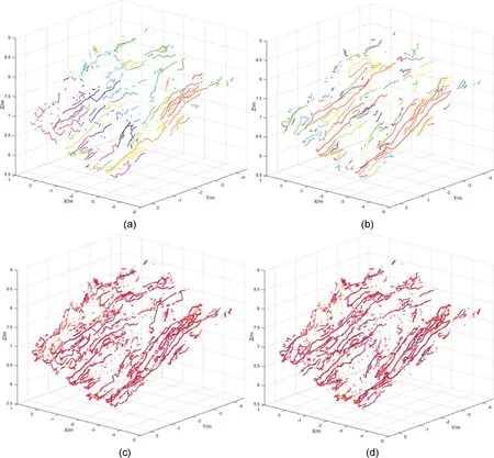
Fig.20. Comparison of trace mapping effect of case B(a)between different methods:(a,c)The traces detected by the growth method;and(b,d)The traces detected by our method.In (a, b), each color represents a trace. In (c, d), blue segments represent detected traces while red points represent feature points.

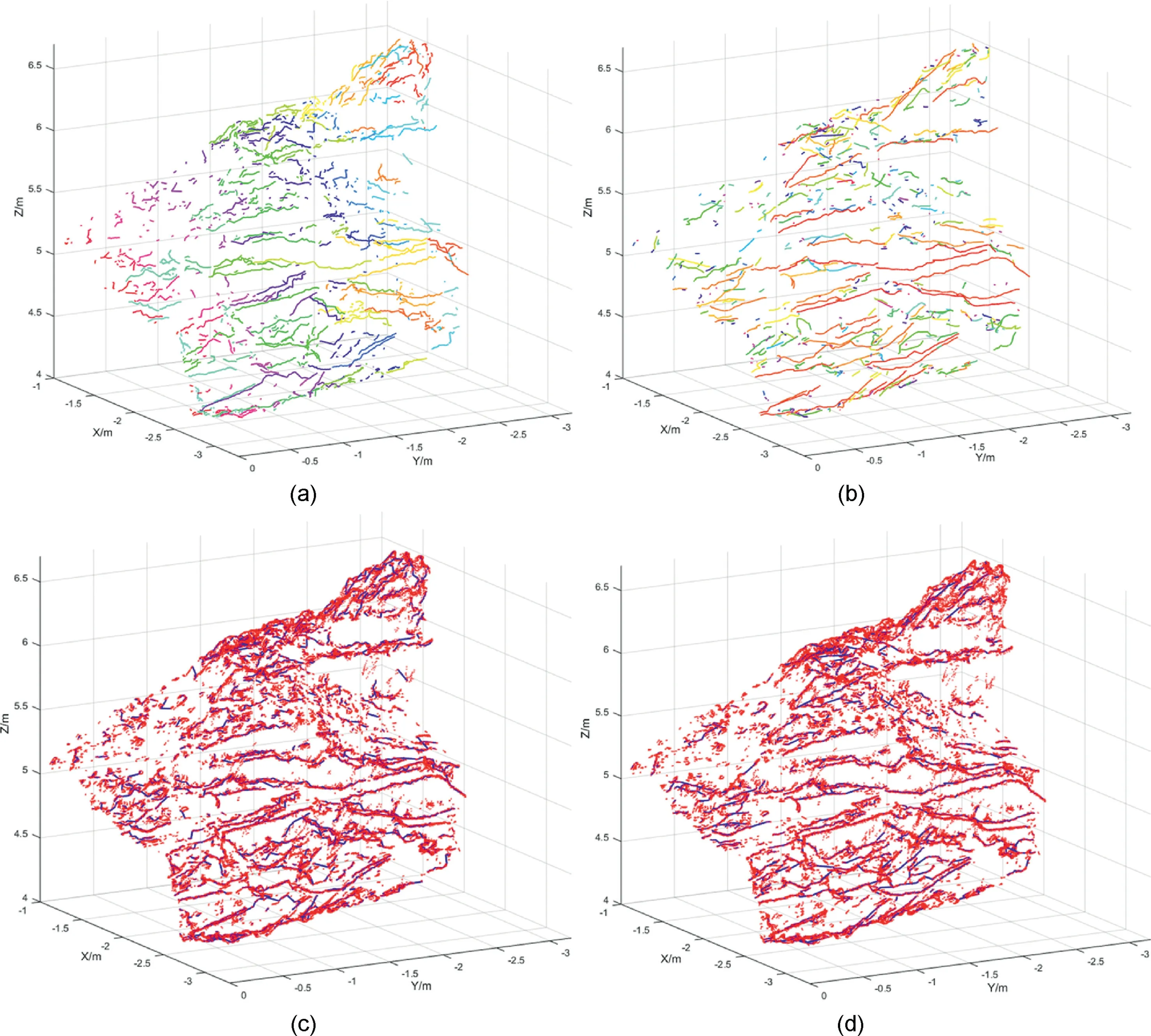
Fig.21. Comparison of trace mapping effect of case B(b)using different methods:(a,c)The traces detected by the growth method;and(b,d)The traces detected by our method.In(a, b), each color represents a trace. In (c, d), blue segments represent detected traces while red points represent feature points.

As shown in Fig. 16b, the mean trace length increases as thresholds ofD,R1or1increase. Because the above three thresholds define the axial, radial and curve extents of trace segment connection, the larger they are defined, the more easily trace segments will be connected. However, too large values ofD,R1and1will falsely connect trace segments which belong to different traces (Fig.18a, c and e) and segments that belong to the same trace cannot be connected effectively if they are defined too small(Fig.18b,d and f).Through data tests based on cases A and B,the optimal value ofDis between 15 and 20 times the average edge length of triangular mesh.The optimalR1is between 6 and 8 times the average edge length of triangular mesh,and1is between 30and 45.

4. Discussion

Li et al.(2016)proposed a growth method of discontinuity trace mapping on 3D digital surface model (DSM). Based on feature points detected by NTV, they detected traces by the procedures of trace feature point grouping,trace segment growth,trace segment connection,and redundant trace segment removal.For comparison,both the growth method and our method were employed to detect traces of case A in this section. Both the methods started with the same feature points generated by NTV and ended with traces finally detected. Mean trace length were calculated using the circular window method which was the same as depicted in Section 3.1.3.

4.1. Comparison of trace mapping effect

As shown in Figs.19e21,the shortcomings of traces detected by the growth method can be summarized as follows: (1) traces are coarse;(2)shapes of traces are easily affected by noisy points;and(3) some trace segments that belong to different traces are connected falsely.

Comparatively, traces detected by our method were smoother and linear because they were composed of contracted feature points that aggregated on skeletons instead of separate feature points that were scattered around traces.Therefore,the contraction algorithm (in Section 2.2) was robust to noisy points and could reflect the principal position of traces accurately.In addition,it can be seen that the false connection of trace segments belonged to different real traces were decreased because the connection algorithm (in Section 2.5) reflected the principal extension trends of trace segments more accurate.

4.2. Comparison of trace mapping efficiency

Both the growth method and our method were programed by MATLAB (2017a version) software and performed on an Intel Core I7-8700k and 16 GB DDR4 RAM. For comparison of algorithm efficiency, we used different point clouds resolution to sample the analyzed regions of both cases B(a) and B(b). As shown in Table 2,the running time of our method is shorter than that of the growth method. As shown in Fig. 22, with the number of feature points increases, the running time of the growth method increases significantly faster than the time increment of our method.

4.3. Parameter settings

Based on the analysis in Section 3, the optimal parameter settings were selected asR02:5L0;065;U0:98;D17:5L0;R15L0and130. The optimal parameter settings were suggested as default parameters, because for all point cloud data tested, the trace recognition results based on the optimal parameter settings were more consistent with that observed from the pictures or the point clouds of the corresponding rock masses than the results of the growth method (Li et al., 2016).

In addition, the parameter settings were influenced by point clouds quality,because parameter settings were dependent on the recognition results and the recognition results were influenced by the point clouds quality.The point clouds quality was interfered by many factors.Plants,shelters of natural rock mass and trivial grains and fractures caused by blasting disturbance of tunnel excavation faces were the disturbance factors when point clouds were obtained directly from laser scanning. When point clouds were obtained from 3D reconstruction based on photogrammetry, light intensity, shadows, dust and even lens distortion of cameras were considered as disturbance factors.

Although there were many factors influencing point clouds quality and the parameter settings,the proposed method based on the optimal or default parameters was more robust than the growth method (Li et al., 2016). The reasons are: (1) For the proposed method, point cloud skeleton extraction (Section 2.2) reduces the interference of noisy points; and (2) Trace segments connection(Section 2.5) considers more about the real extending trend of traces than the growth method.

In conclusion, there is no need for the proposed method to select new parameters when every time encountered a newrock mass, for the optimal or default parameters have served well for trace recognition based on point cloud data we have had. We suggest reselecting the parameters only when the results exceed the users’ expectation or specific results that the users need.

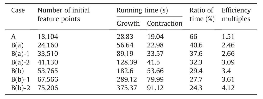
Table 2CPU time. For clearer comparison, cases B(a)-1 and B(a)-2 are generated from case B(a) using different point clouds sampling resolutions, which is the same as cases B(b)-1 and B(b)-2.

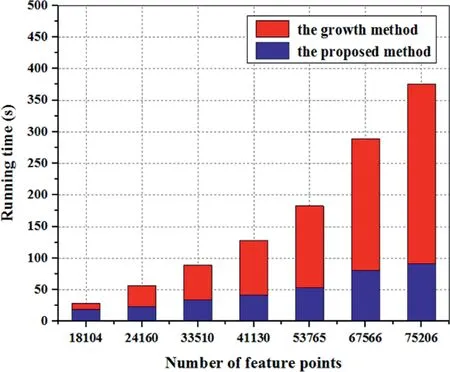
Fig. 22. Comparison of running time.

5. Conclusions

This paper proposed a new method for trace mapping based on 3D point clouds of rock mass surfaces. Features points were generated by NTV first, and then the proposed method was performed to detect traces. Compared with the growth method, our method (trace feature points contraction, trace feature points connection, trace segments linearization, and trace segments connection) performed two principal advantages: (1) Trace mapping result was more accurate because the detected traces were smoother, more linearly outstretched and more robust to noisy points, and the detected traces could better match the principal trends of the real traces; and (2) The proposed method was more efficient and the enhancement of efficiency was more remarkable as the number of feature points increased.

A sensitivity analysis was conducted to identify the optimal parameters of the proposed method. In our cases, the optimal threshold radiusR0in contraction algorithm was 2e3 times the average edge length of triangular mesh. The optimal threshold angle0in feature point connection algorithm was 60e70. The optimal linearization thresholdUin trace segment linearization algorithm was 0.96e0.98. In trace segment connection algorithm,the optimal threshold distanceDwas 15e20 times the average edge length of triangular mesh.The threshold distanceR1was 6e8 times the average edge length of triangular mesh,and threshold angle1was 30e45.

The case study indicated that the proposed method provided more efficient and accurate measurements of discontinuity geometric parameters.As a supplement to traditional measurement of discontinuity traces,the proposed method could achieve quick and accurate trace mapping in engineering fields. The results of the proposed method can be used to (1) calculate the tunnel surrounding rock quality indices such as rock mass rating (RMR)(Bieniawski,1989)andQvalue(Barton et al.,1974),(2)evaluate the rock mass blasting disturbance during tunnel excavations, (3)divide units of tunnel surrounding rock block units, (4) construct models of geological bodies (ISRM,1978), and (5) serve for mechanism analysis of tunnel surrounding rock (Zhu et al., 2016).

Declaration of Competing Interest

The authors wish to confirm that there are no known conflicts of interests associated with this publication and there has been no significant financial support for this work that could have influenced its outcome.

Acknowledgments

This work was supported by the Special Fund for Basic Research on Scientific Instruments of the National Natural Science Foundation of China(Grant No.4182780021),Emeishan-Hanyuan Highway Program, and Taihang Mountain Highway Program.