
Utilization of Extrinsic Fabry-Perot Interferometers with Spectral Interferometric Interrogation for Microdisplacement Measurement
2020-05-14 01:23:22LeonidLiokumovichAleksandrMarkvartNikolaiUshakov
Leonid Liokumovich|Aleksandr Markvart|Nikolai Ushakov
Abstract—The paper presents a number of signal processing approaches for the spectral interferometric interrogation of extrinsic Fabry-Perot interferometers (EFPIs).The analysis of attainable microdisplacement resolution is performed and the analytical equations describing the dependence of resolution on parameters of the interrogation setup are derived.The efficiency of the proposed signal processing approaches and the validity of analytical derivations are supported by experiments.The proposed approaches allow the interrogation of up to four multiplexed sensors with attained resolution between 30 pm and 80 pm,up to three times improvement of microdisplacement resolution of a single sensor by means of using the reference interferometer and noisecompensating approach,and ability to register signals with frequencies up to 1 kHz in the case of 1 Hz spectrum acquisition rate.The proposed approaches can be used for various applications,including biomedical,industrial inspection,and others,amongst the microdisplacement measurement.
1.Introduction
The extrinsic Fabry-Perot interferometer (EFPI)is the modification of an optical Fabry-Perot interferometer,formed by two reflecting surfaces.There are two types of EFPIs distinguished by the intra-cavity media:
1)Air-gap,where the Fabry-Perot cavity is formed by the fiber end(with the typical reflectivity about 3.5% for the wavelength range of 1.55 μm)and an external mirror,either opaque or semi-transparent(in this case several interferometers can be serially multiplexed);
2)Wafer-based,where the Fabry-Perot cavity is formed inside the transparent plate of some materials and the reflection occurs at the plate faces.In this case,the reflectivity can be increased,while the light losses inside the cavity can be decreased due to the smaller beam divergence in media with a greater refractive index.
Generally,in EFPI,the intensity of the reflected light is registered,demonstrating an oscillating relation to the interferometer baselineLdue to interferometric effects[1].Such a short-baseline interferometer is highly convenient for measuring different physical quantities.
Sensors based on EFPI have been a subject of an extensive study of both academia and industry for the last two decades[2].Their advantages,including immunity to electromagnetic radiation,low cost,small dimensions,ability to operate in Harsh environments,multiplexing capabilities[3],and high performance,make them attractive for the wide range of applications for measuring temperature[4],strain[5],pressure[6],humidity[7],electric field[8],and microdisplacements[9],[10]in such areas as oil and gas exploitation[6],structure health monitoring[5],nuclear power industry[11],and others.
There are two basic classes of the EFPI baseline measurement techniques:Tracking only the baseline variations and capturing the absolute baseline value,which include conventional white-light[12]techniques utilizing a tunable read-out interferometer and approaches based on the registration and subsequent analysis of the interferometer spectral function (wavelength-domain interferometry).The variation-tracking approaches are characterized by relatively high operational frequencies and resolution[13],however,their disadvantage is the uncertainty of the initial value,which is crucial in many tasks.One of the most accurate spectral registering methods is frequency scanning interferometry which is known for the picometer-level resolution,high absolute accuracy,and wide dynamic measurement range[9].
In this paper we present signal processing techniques,enabling one to enhance the measurement resolution for the wavelength-domain interrogation of EFPIs in the cases of both a single sensor and multiplexed sensors.Furthermore,an algorithm,enabling one to capture the absolute value of the fast EFPI baseline oscillation in the case of the wavelength-scanning interrogation,is proposed.An experimental demonstration of these techniques is also presented;the attained baseline resolution is discussed.
2.General Provisions
Strictly speaking,the spectral transfer functionS(λ)of the Fabry-Perot interferometer is defined by the Airy function[14].In the case of the reflected light from the interferometer,it can be expressed as follows:
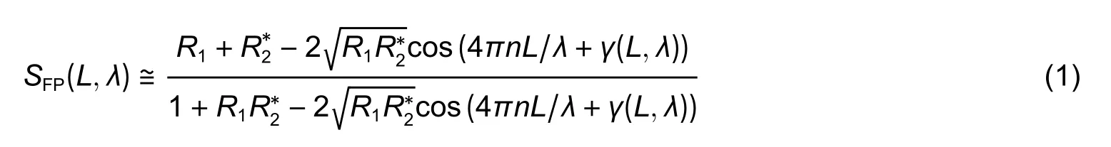
which,in the case of the low finess interferometer,is simplified to the following form:
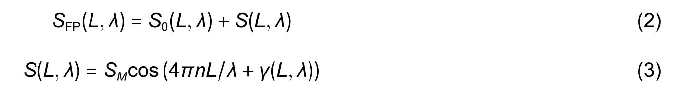
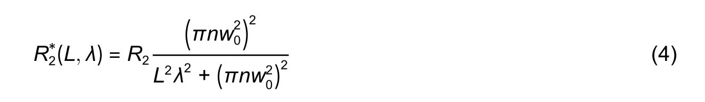
and the additional phase is expressed as
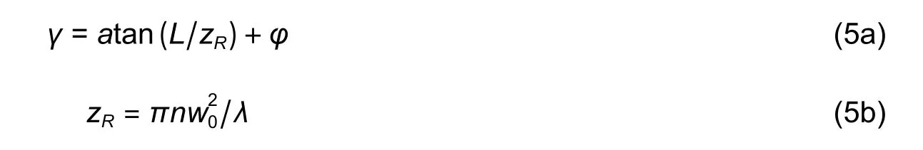
whereR2is the reflectivity of another mirror,ais a constant,andw0is an effective radius of a Gaussian beam at the output of the first fiber,close to the fiber mode field radius.φis an additional phase shift,induced by the mirror(typicallyφ=πfor the light reflected back to a less optically dense medium from a bound with a more optically dense medium).
Therefore,the shape of the interferometer spectral function is unambiguously related to its baseline,which can be found by applying special signal processing techniques to the measured functionS′(λ).One of the most advanced approaches is to approximateS′(λ)with(1)or(3),providing an estimate of the interferometer baseline with extremely high resolution and accuracy,which are limited by the precision of the utilized spectral analyzer.
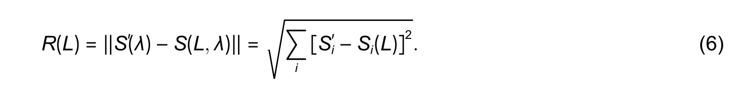
In order to find the interferometer baseline from its measured spectral function,one has to solve the leastsquares minimization of a residual norm:
3.Signal Processing
In the current section,several signal processing approaches for the EFPI sensors interrogation by means of frequency scanning interferometry are described.The classification used below embraces two criteria:The number of sensors interrogated (a single sensor/multiplexed sensors) and the type of the sensor signal acquired(static/dynamic).Such classification covers all the main sensing tasks in the state-of-the-art systems.The case described in subsection 3.1(a single sensor with static perturbations)is the most fundamental and is utilized in all the following approaches.However,the case of multiplexed sensors with dynamic perturbations is not considered below since it can easily be derived from the approaches described in subsections 3.2 and 3.3.
3.1.Single EFPI for Static Signals
According to[9],the approximation task in its direct form requires a great number of calculations,therefore,it cannot be implemented in a real-time mode.A significant enhancement can be attained if a simple pre-estimation based on fringe-counting is used:
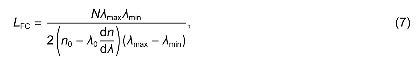
whereλ0is the central wavelength of the analysis,n0is the mean refractive index at the analyzed spectral range,Nis the number of oscillations of the measured spectrum on the analyzed spectral range,andλmaxandλminare the bounds of the analyzed spectral range.In(7)the dispersion of the intra-cavity media is taken into account to avoid abrupt errors.This pre-estimationLFCcoincides with the actual baselineL0within~10 μm,depending on the interrogator parameters.For further improvement of the approximation algorithm,theR(L)function behavior should be analyzed.As in[9],it has a quasi-periodic structure with the global minimum at the pointL0and the local minima at pointsL0±kλ0/2n0withkbeing an integer.Therefore,finding the position of theR(L)minimum nearest toLFCwill result in one of the lateral minima,located atkλ0/2n0away from the global minimum.
The proposed signal processing algorithm can be divided into four stages.At the first stage,the preliminary estimate of the cavity length is provided.Three following steps are developed in order to reduce the search domain to several narrow intervals,thereby extremely increasing the performance of the proposed method.The initial step of the search algorithm is decreased at each stage,providing increasing accuracy of theR(L)extreme point localization.
The proposed algorithm is described below in more detail.
1)The preliminary value of the cavity lengthLFCis found according to the number of the measured spectra oscillation periods by(3).
2)The preliminary valueLFCis specified with higher accuracy by the use of the binary search algorithm(BSA).The summation in(6)is performed over the spectra pointsIsel1defined in[9].The initial value is set toLEand the initial step is set toλ0/8.The search is terminated afterm0BSA stages are performed and the step becomes less thanλ0/2m0+3.Thus,the extreme pointL1located in the interval[LE–λ0/2,LE+λ0/2],with precision aroundλ0/2m0+3,is reached.The optimal value form0is about 7 to 8,which provides the estimation accuracy of the cavity length of about 1 nm.
3)At the second step,the coordinate of one of theR(L)minimums is found(maybe,local).However,taking into accountS(L,λ)features,one can derive a set of the possible coordinates of the global minimum.Therefore,the pointsL2,k=L1+kλ0/2,∣k∣≤kmax,are taken as the initial values for the third stage and thekmaxvalue depends on the number ofS(L,λ) oscillation periodsNos.The coordinates of the extreme points are adjusted using BSA,converging them to the resulting pointsL3,k.For each of them,the residual norm is equal toRk=R(L3,k).So,the minimal value of the residual normRk0corresponds to the valueL3,k0best corresponding to the desired cavity length value.
4)At the last stage,the valueL3,k0is adjusted using BSA,which provides the final resultLR.
As will be discussed in Section 4,this approach dramatically increases the accuracy and performance of signal processing,resulting in the picometer-level resolution of the EFPI baseline.
3.2.Single EFPI for Dynamic Signals
As was mentioned above,the sample rate of the conventional wavelength-domain interferometry measurement is equal to the spectrum acquisition rate,which does not exceed the level of several Hz.In the current section,we propose a method for registering more rapid fluctuations of the interferometer baseline.Let us assume that the wavelength-scanning interferometry methods are used for interrogating the sensor,therefore,at each particular temporal momentti∈[–TM/2,TM/2](or theith spectrum point),the wavelengthλican be written asλi=λ0+kλti,wherekλis the wavelength scanning rate andTMis the length of the temporal interval of the spectrum acquisition.It should be noted that the zero-time momentt=0 corresponds toi=0(the middle point of the spectrum)and the step betweentimoments is equal to 1/fD,wherefDis the sample rate of the acquired photodetector signal.
For further convenience,we change the wavelengthλito the optical frequencyνj=ν0+kνtjwithν0being the frequency corresponding to the central wavelengthλ0andkνbeing the frequency scanning rate in the EFPI spectrum expressions,as it was done,for instance,in [15].It should be noted that the uniform grids of the wavelengthsλiand the optical frequenciesνjdo not correspond to each other,since the uniform wavelength stepping withΔproduces a non-uniform frequency grid(νi=c/nλi),and vice versa.Hereinafter,the indexiwill define the uniform wavelength grid,and the indexjwill define the uniform frequency grid.Taking into account the baseline variations:

whereδLj=δL(tj)represents the OPD variations,taking place during the spectrum acquisition.Using the optical frequency notation,we convert the expression for the interferometer spectral function to the following form[16]:
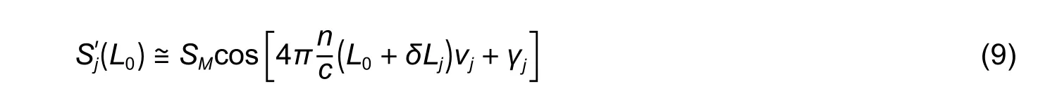
wherecis the speed of light in vacuum.
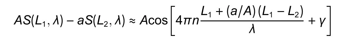
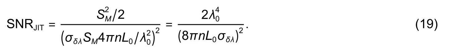
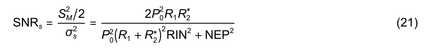
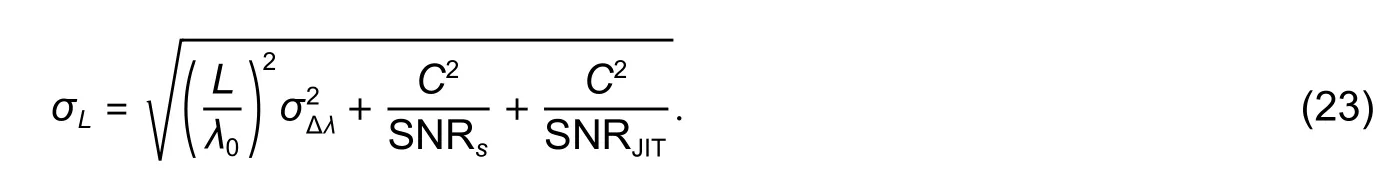
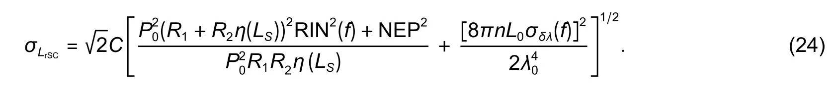
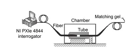
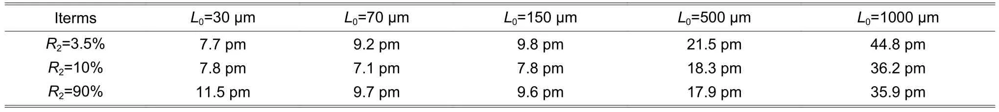
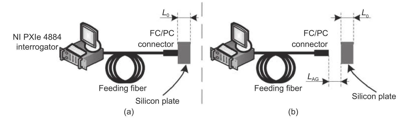
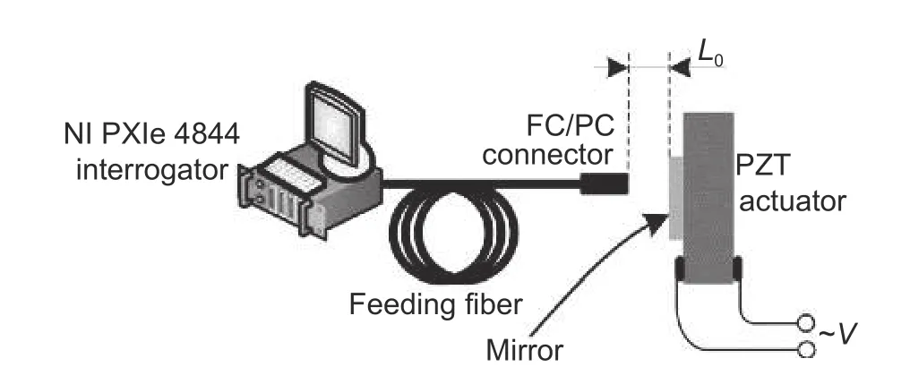
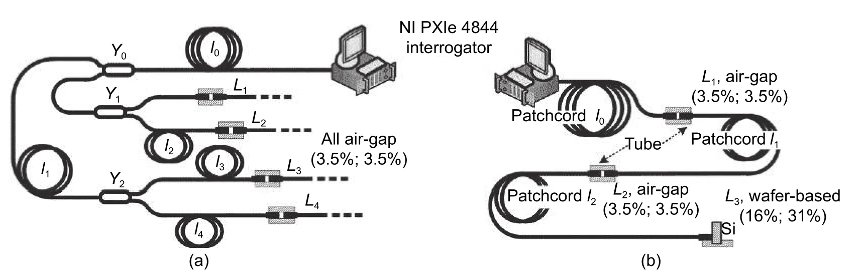
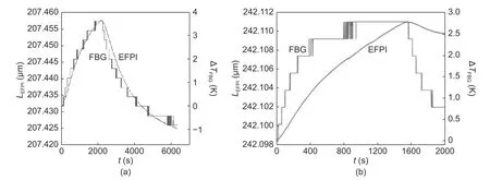
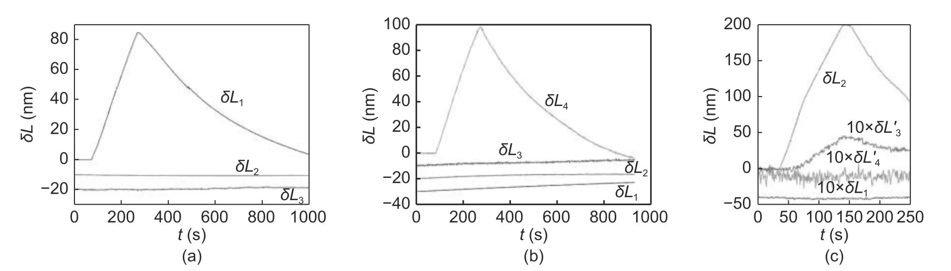
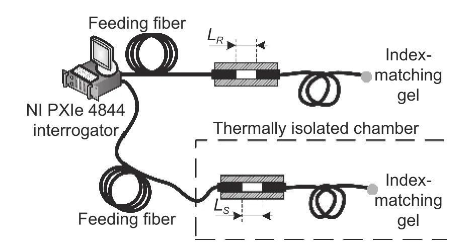
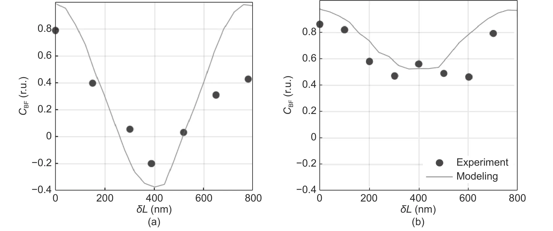
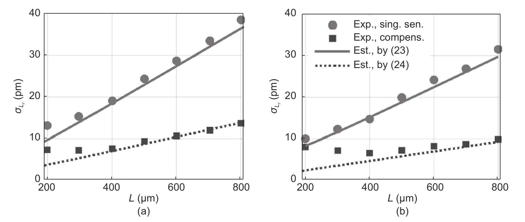
Equation (9)corresponds to the angular-modulated signal with respect toνj,where the regular argument increment is provided by the mean baselineL0and its deviations are stipulated byδLjand the additional argument deviationγj.Taking into account the weak dependencyγj(L) and assuming thatδLj< Following(9),signal processing for obtainingδLjfrom the measured spectrumcan be divided into the two following stages. 1)Find the average baseline valueby approximating the measured spectrumas discussed in subsection 3.1.In the context of the frequency detection task,the first step is essential for finding the “carrier frequency”,necessary for further demodulation of the baseline variations.In the temporal representation ofspectrum,its carrier frequency can be expressed as 2)By means of the Hilbert transform,one can calculate the analytical signal for the measured spectral functionAfter that,the argument of the analytical signal is obtained to which the standard unwrapping procedure,based on the Itoh-criterion[17]is applied.Thus,the continuous argumentψjis derived.Then the desired difference of the arguments is calculated as from which the baseline variationδLjcan be found,according to the following expression: With the use of the first step,L0is obtained with very high accuracy,which enables one to find the nonperturbation part of theψjargument with much greater precision in comparison with the method of detrendingψjor other simple methods of deleting the regular components ofψj. It should be noted that in practical optical spectrum analyzers,the uniform wavelength grid is generally used.Therefore,the corresponding optical frequency scaleνiin (9) will be related to temporal moments asνi=c/(λ0+kλti),resulting in an incorrect calculation of the analytical signals’ phases and therefore,leading to improper performance of the signal processing.In order to overcome this problem,two possible solutions can be proposed: a)Utilization of non-uniform fast Fourier transform(NUFFT)algorithms[18]for the analytical signal calculation; b)Interpolation of the initially registered spectrumS′(λi) with the uniform wavelength scale to spectrumS′(c/vj)with the uniform frequency scale before the analytic signal calculation.The inverse interpolation will be needed for the calculatedδLjsignal in order to obtain the signalδLi(and),uniformly sampled with respect to time. After calculating the baseline variation with uniform temporal samplingδLi,it can be filtered by a low-pass filter with the cut-off frequencyfSc.The reason for doing so is the following:On the one hand,the frequency of registeredδLiis limited byfScand,on the other hand,the sample rate ofδLiis again equal tofD,which is usually much higher than the working frequency band. It should be noted that for the proper operation of signal processing mentioned above,the spectral components of thetemporal representation must not decrease below zero and satisfy the Nyquist limit,i.e.the argumentψjcan be calculated.For simplicity,let us consider the limitations in the case of harmonic oscillation of the interferometer baseline with amplitudeLmand frequencyfL,δLj=Lmcos(2πfLtj). According to (3),the oscillation period of the EFPI spectral function is strongly related to its baselineL0.Therefore,if several EFPIs with different baselines are embedded in one fiber line,the overall transfer function of such system will contain a superposition of quasi-harmonic signals in(3)with different frequencies and therefore,can be expressed as whereH(L1,L2,…,LN,λ)contains the quasi-static component and a number of parasitic components,with the baselines different fromL1,L2,…,LNand must be filtered out;the amplitudewill be discussed in detail later on.Therefore,extracting partial spectraSk(λ)and applying the baseline demodulation approach developed for a single sensor (see subsection 3.1),one can obtain the readings from each multiplexed sensor. In a parallel configuration,the light intensity brought to each interferometer is determined by the division ratios at the coupling elements.In the simplest case of the uniform power distribution between the sensors,the corresponding amplitudecan be expressed as whereR1,kandR2,kdenote the reflectivities of mirrors,forming thekth interferometer. In order to minimize the variance of,a nonuniform distribution of the light power over the sensors can be used,in this case,the estimation of (15)must be modified.The lengths of the feeding fibers must be sufficiently different in order to suppress parasitic interference signals,therefore,the componentH(λ)in(14)will be stipulated only by the higher harmonics of the Airy function ((3)contains only the first harmonic of the Airy function). In a serial scheme,the interferometers are connected to the sensor interrogator one after another,therefore,when considering the signal of thekth interferometer,the light propagation through the preceding interferometers must be taken into account.The spectrum of the light,reflected from thekth EFPI,can be written as whereST,i(λ)is spectrum,transmitted by theith interferometer,therefore,the expression forcan be written in the following form[3]: Thus,an assumption of the Gaussian profile of the free-space(inside the interferometer)and the fiber modes was made,allowing us to approximate the power coupled from the free-space beam to the fiber mode as proportional to squared modes radii.According to our experimental results,these assumptions are valid in the case ofL>200 μm.However,in practice one might utilize sensors with smallerLvalues(see Section 4);and in this case,the valuescalculated according to(16)will be underestimated. BecauseST,1(λ)is quite similar to (3),its oscillating part does not affect the mean optical power and it will modulate the light spectrum brought to thekth sensor,which will result in the uprising of parasitic components of the formaSk(λ)ST(Lj,λ),j Therefore,the main origin of the cross-talk in the systems considered in the paper is the coincidence of the oscillation periods of the parasiticH(λ)and the targetSk(λ)components in(14).In order to avoid the cross-talk,the following condition on the cavity lengths must be fulfilled: wherepandqare integers,in the worst casesp=2,q=0 orp=±1,q=±1,|i–j|=1;ΔL=λ02/2nΛis the step in the interferometer baseline domain after the application of Fourier transform to theS(λ)function andΛ=λmax–λminis the width of the spectral interval of analysis.Considering the sum of target and parasitic quasi-harmonic signals of(3)with close frequencies and significantly different amplitudesAanda,we obtain with the resultant error written as follows: The values ofAandacan be analyzed separately,which is out of the scope of the current paper,however,for the practical case ofa/Abeing about 0.01 andδLbeing about 100 nm,the resulting deviation of the registered baseline from the real one will be about 1 nm,which is around an order larger than the achievable displacement resolution(see subsection 4.4 below). Therefore,the system of multiplexed EFPI sensors must be carefully designed in order to avoid the cross-talk between the sensors,on the one hand,and allow sufficient spacing between theSk(λ)components for them to be distinguished by the bandpass filter,on the other hand. An extensive study of the single EFPI displacement sensor resolution limits with the wavelength-scanning interrogation was done in[20]and[21].It was shown that the main noise sources are including: 1)The absolute wavelength scale shift Δλ0,which is determined by the fluctuations of the triggering of the scanning start, 2)The jitter of the wavelength pointsδλi,caused by the fluctuations of the signal sampling moments, 3)The additive noiseδsi,produced by the photo registering units,light source intensity noise,etc. These mechanisms will result in the distortion of the registered interferometer spectral functionS′(λ).Therefore,the spectrum approximation procedure gives an erroneous result,denoted throughout the paper asLa.When considering a vector of consequently measured baseline values,its standard deviationσLacan be calculated.Generally,σLais used as a quantitative characteristic of sensor resolution which is approximated as 2σLa. The first mechanism provides the shift of the measured interferometer spectrum,inherently shifting the displacement sensor readings as follows: The jitter of the spectral points during the interrogation produces the distortion of the measured spectral functionS′(λ).This distortion can be interpreted as additive noise with some variances.The resulting signal-to-noise ratio SNRJITcan easily be estimated by simple trigonometric derivations[20]: Considering the third mechanism,one has to take into account that generally the noise variance can depend on the mean optical powerPI,incident to the photodetector(the shot noise level and laser intensity noise influence are strongly related to the mean power level).The dependency can be adequately approximated by a power function as which,for EFPI,produces the signal-to-noise ratio of the spectrum,written as whereP0is the optical power irradiated by the light source;is the effective mirror reflectivity,taking into account light losses due to the divergence of a non-guided beam inside the cavity.RIN is a parameter characterizing laser intensity noise and NEP characterizes the thermal and electronic photodetector noise. The influence of the additive noise on the standard deviation of the baseline measurement can be found either by the numeric simulation,or analytically using the Cramer-Rao bound.It can be shown that for the approximation approach[9],the corresponding relation can be written as whereCis within the interval of 9×10⁻⁴μm–1to 11×10–4μm–1for different parameters of the considered OPD demodulation approach. Finally,the expression for the baseline standard deviation can be obtained by combining (5)and (22)and taking into account the variance summation rule: Substituting(3),(5),(19),and(21)to(23),one will be able to obtain the final explicit expression,which is not done due to excessive bulkiness. Throughout the paper the following noise compensations scheme will be assumed:Two interferometers with similar parameters are used for the measurement,one of them is exposed to the target perturbation(which is the actual measurand)and will be referred to as the sensing or signal interferometer,and the second one is isolated from any environmental changes and will be referred to as the reference interferometer.The interferometer baselines will be denoted asLSandLR,respectively.Both these interferometers will be assumed to be interrogated by the same tunable laser,while their spectral functions will be registered by independent (although,similar)photodetectors. Considering the task of noise compensations,one needs to determine the likelihood of the two interferometers’ measured baselines fluctuations,which can be done by means of the correlation coefficient.Therefore,in order to study the ability of noise cancellation,one needs to study the behavior of the correlation coefficientCBFbetween the registered baseline values of the reference and sensing interferometers with respect to the mechanisms,mentioned in subsection 3.4. As can be seen from(18),the absolute shift of the wavelength scale produces an error,proportional to the baseline value,therefore,its influence will be correlated for the signal and reference interferometers with arbitrarily different baselines. Considering the impact of individual spectral points jitter,one has to take into account that it is indirect in nature:Jitter itself produces equivalent additive noise,which,in turn,affects the accuracy of the approximation procedure[9].If the sensing and reference interferometers have equal baselinesLS≈LR,the shapes of their spectral functions will be the same,resulting in identical noise patterns,produced by jitter.This will provide equal baseline measurement errors for both interferometers andCBF=1.Recall the properties of the spectral functionS′(λi),particularly that it is quasi-harmonic with a period close toλ0/2,one can expect secondary maximums of correlation in the cases of |LS–LR|=λ0/2 and |LS–LR|=λ0/4(when interferometers spectral functions are nearly inversed).On the other hand,for arbitrarily different baselinesLSandLR,the spectral functions will be uncorrelated,producing sufficiently different noise patterns,which will result in uncorrelated baseline noise.The dependency of the produced baseline noise correlation on the difference of interferometer baselines can be found by means of the numeric calculations. Considering the additive noise (the third mechanism),one needs to take into account the two main sources—laser intensity noise,equal for the both interferometers,and photodetector noise which is produced by different devices and hence uncorrelated,producing uncorrelated errors.Laser intensity noise,being the same for the measurement and reference interferometers,will produce identical errors in the case of close baseline valuesLS≈LRand |LS–LR|=λ0/2.In the case of |LS–LR|=λ0/4,the influence of laser intensity noise will be inverse for the signal and reference interferometers and will produce anti-correlationCBF(λ0/4)=–1.For arbitrarily different baselines,the baseline fluctuations will be uncorrelated,CBF=0.The dependencyCBF(LS–LR)for a particular setup will depend on the relation of the above mentioned noise sources. In an ideal case of equally adjusted interferometers OPDs,the influences of both laser intensity noise and wavelength scale shift on the measured OPDs will be totally compensated,with no affection on the fluctuations of the measured OPD values after noise compensations,denoted asLrSC.For the estimation of resolution attainable in t√h is case,let us substitute into(23)the following parameters:σΔλ=0,usinginstead ofσδλ,RIN=0,and usinginstead of NEP(two photodetectors will produce independent additive noise and wavelength points jitter of the same level,the impact onσLrSCwill,therefore,be stipulated by the doubled variance of a single detector influence).In such a manner,(23)is modified to the following form: In order to study the exact dependency of the signal and reference interferometers’ baseline noise correlationCBFon the baseline difference,a numeric simulation has been performed.Two spectral functionsS(LS,λ)andS(LR,λ)were calculated according to(1),the differenceδL=LS–LRwas varied within the interval of 0 to 0.8 μm,the valuesLSandLRthemselves were around 200 μm.The rest parameters were chosen close to the experiment:Wavelength scanning range from 1510 nm to 1590 nm and interval between spectral pointsΔ=4 pm,resulting inM=20001 points in the spectrum;wavelength jitter standard deviationσδλ=1 pm;scale shift standard deviationσΔλ≈0.05 pm;laser output optical powerP0≈0.06 mW;RIN in the full frequency band 60 dB(in the case of~1 MHz photodetector band corresponding to the practical 120 dB/Hz1/2RIN spectral density);photodetector NEP=30 nW in the full frequency band (3×10–11W/Hz1/2for~1 MHz photodetector band).For all baseline combinations ofLSandLR,an ensemble ofN=100 realizations of noise was calculated for the better statistical validity of the simulation results.The correlation coefficientsCBFof the resulting vectors of the baseline fluctuations were calculated.The simulated dependencyCBF(δL)demonstrates that in the case of interferometers’ OPD difference less than 50 nm,noise compensations can be performed. The approaches proposed in the paper were implemented and tested experimentally.The experimental setups cover the most relevant and widely used EFPI configurations;the additional classification in the class of a single sensor with static perturbations is stipulated by some peculiarities and differences in applications of air-gap and wafer-based interferometers.Spectra measurement was carried out with the help of the optical sensor interrogator National Instruments(NI)PXIe 4844,installed into PXI chassis PXIe 1065 and controlled by PXIe 8106 controller.The spectrometer parameters are the followings:The scanning range is from 1510 nm to 1590 nm (spectral interval widthΛ=80 nm),the spectral stepΔ=4 pm(the number of spectral pointsM=20001),the scanning speedkλ=2400 nm/s,the spectrum acquisition timeTM≈0.035 s,and the output powerP≈0.06 mW. The interferometer under consideration was formed by two fiber ends packaged with PC connectors,fixed in a standard mating sleeve.The air gapL0between the fiber ends varied from~30 μm up to 5 mm by the use of Standa 7TF2 translation stage.The experimental setup is shown in Fig.1. Fig.1.Experimental setup for static signal measurement of single EFPI. The left fiber was rigidly screwed to the sleeve,while the right one was fixed by the friction in the tube.The right fiber was connected to the translation stage only at the moments ofL0adjustments and then unhooked in order to eliminate the influences of the stage’s possible mechanical vibrations.Three combinations of the fiber ends reflectivity were used:Both mirrors are 3.5%(Fresnel reflection at the glass-air boundary);3.5% and~10%(the increased reflectivity was produced by dielectric evaporation on the fiber end);3.5% and~90%(opaque aluminum mirror,glued to the fiber end).The interferometer was placed in a thermally isolated chamber in order to estimate the intrinsic limits of the measurement resolution.For the same reason,the far end of the right fiber was put in the index-matching gel to avoid parasitic reflection. The final stage of the experimental study was to investigate the resolution of the baseline measurement.Spectra measurement was carried out for about 10 minutes for eachL0value,resulting in 600 spectraperL0point(iis the number of spectral points andkis the number of spectra).LRkvalues were estimated with the use of the approach described in subsection 3.1 for each acquired spectrum,k=1,2,…,600.The resulting standard deviationsσLr(LR),calculated forLRk,are shown in Table 1. Table 1:Baseline standard deviations for different baselines and R2 values The interferometer studied in the current section was formed by the fiber end and the crystalline silicon wafer.The experiments of two types were performed:With the silicon plate tightly adjacent to the fiber end and with the air-gap left between the silicon plate and the fiber,thus,the remote testing of the wafer was performed.The thicknesses of the utilized silicon wafers were about 240 μm and 471 μm.Both experimental configurations are shown in Fig.2. Fig.2.Experimental setups for the cases of(a)contact and(b)remote measurement of the silicon wafer thickness. As for the air-gap interferometers,spectra measurement was performed for about 10 minutes for eachL0,resulting in 600 spectrafor each wafer thickness.Interferometers were placed in the thermally isolated chamber in order to eliminate the influence of environmental fluctuations.For the contact configuration,LRkvalues were estimated with the use of the approach described in subsection 3.1 and with the dispersion of silicon taken into account.The silicon refractive index was approximated by Sellmeier equation[22].In the case of the remote configuration,the additional parasitic OPDs,induced by air-gap,occurred.Therefore,the approach,similar to the one described in subsection 3.3,was applied.As a result,similar resolution of wafer thickness measurement was attained in both configurations:~10 pm for the 240 μm plate and~21 pm for the 471 μm plate. The interferometer under study was formed by the fiber end packaged in an FC/PC connector and an external metallic mirror(~90% reflectivity),adjusted to the piezo ceramic actuator.The controlling voltage for PZT was generated by the PXIe 5421 signal generator,installed in the same PXI chassis as the used sensor interrogator PXIe 4844.The experimental setup is schematically shown in Fig.3. Fig.3.Experimental setup for dynamic signal measurement from single EFPI. The efficiency of the PZT actuator was approximately 100 nm/V within the frequency range of 10 Hz to 1000 Hz.The mean baseline value was varied from~500 μm to~750 μm,resulting in thecarrier frequencyfSc≈940 Hz to 1400 Hz(see(10)).The parameters of the PZT supplying voltage were the followings: 1)The peak-to-peak amplitude was varied from 0.1 V to 6.0 V,resulting in the peak-to-peak value of the EFPI baseline variations from 20 nm to 1.2 μm; 2)The frequency was varied from 50 Hz to 1000 Hz; 3)The oscillation shape was either harmonic or triangular. In Fig.4,the spectra of the registered baseline oscillations of the amplitudes from 15 nm to 90 nm and frequencies 200 Hz and 800 Hz for the mean interferometer baselineL0≈550 μm are shown.Estimating the baseline resolution as the double median level of spectra,the baseline oscillation resolution of about 4 pm/Hz1/2was attained. Fig.4.Spectral density of the measured baseline oscillations for L0≈550 μm. Both parallel and serial multiplexing schemes were implemented experimentally;the experimental setups are shown in Figs.5 (a)and(b),respectively.The parameters of the optical setups were the following:In the parallel schemeL1=41 μm,L2=195 μm,L3=526 μm,andL4=719 μm;in the serial schemeL1=42 μm andL2=170 μm (one fiber end was evaporated,producing greater reflectance),L3=250 μm(silicon plate);the resulting reflectivity shown in Fig.5. Fig.5.Experimental setups for(a)serial and(b)parallel multiplexing configurations. Signal processing was done on a PXI chassis controller.In order to simplify processing,we assumed that the baselines are initially known with accuracy~30 μm.Therefore,the partial element spectraSk(λ)could be extracted by the pre-defined band-pass filters,which was done in the same way as in[23].After that,for eachSk(λ)spectrum th e approximation-based approach for single EFPI described in subsection 3.1 was applied.The standard deviations of the estimated baselinesσLr,shown in Table 2,were calculated over the temporal intervals of about 10 minutes,corresponding to 600 baseline samples for each sensor. Table 2:Standard deviations of the baseline measurement for the serial and parallel multiplexing configurations In order to test the ability of the designed sensors to measure practical physical quantities,a series of experiments were performed.Along with single EFPI air-gap and silicon wafer-based sensors,both multiplexed configurations were tested for their sensitivity to the outer temperature.For this reason,the examined interferometer was placed in the chamber,which was first slowly heated and then cooled.A fiber Bragg grating(FBG)temperature sensor was placed in the same chamber to provide the temperature calibration.In Fig.6,the readings from the 207 μm air-gap(Fig.6(a))and 240 μm wafer-based(Fig.6(b))EFPI sensors,compared with the FBG sensor indications(calculated by the standard software supplied with the interrogator)are shown.The difference between the readings of FBG and silicon-plate sensors is due to the greater thermal inertness of the relatively bulky plate,and hence,different heating rates of FBG and the silicon wafer. Fig.6.Temperature dependency of EFPI baseline for(a)207 μm air-gap and(b)240 μm wafer-based EFPI sensors. The temperature sensitivity of baselines can be approximated to~7.3 nm/K with the corresponding temperature resolution of~2 mK for air-gap EFPI and to~4.4 nm/K with the corresponding temperature resolution of~4.5 mK for silicon wafer-based EFPI. The same experiment was carried out for multiplexed systems.Thus,we consequently heated and cooled one of the sensors,while the rest were placed into the thermally isolated chamber.This operation was repeated for both configurations and all combinations of heated/isolated sensors.In Fig.7,the corresponding baseline curves are shown.Fig.7(a)shows heating of the fourth sensor in the parallel scheme and Fig.7(b)shows heating of the first sensor in the serial scheme.Curves of the deviations of non-perturbed sensors baselines demonstrate no correlation with the perturbed ones,hence,there was no cross-talk in the current systems,at least,at the levels limited by the sensors’ resolution. In a separate experiment with the parallel scheme,L3was changed to~390 μm to match the doubledL2.So,the cross-talk effect(δL2influencing the third sensor readings)was demonstrated by heating the second sensor.The initial values and additional shifts were subtracted from the curves for better representation.For the same reason the curves ofL1,L3,andL4variations in Fig.7(c)were 10 times magnified.The parasitic deviation ofL3shown in Fig.7(c)is in accordance with(17). Fig.7.Temperature measurement by the system of multiplexed EFPIs and cross-talk demonstration:(a)3 multiplexed sensors,no cross-talk,(b)4 multiplexed sensors,no cross-talk,and(c)4 multiplexed sensors,cross-talk demonstration. In order to support the theoretical results,an experimental study of EFPI displacement sensor resolution was carried out.The sensing and reference interferometers were formed by the two ends of SMF-28 fiber packaged with PC connectors,fixed in a standard mating sleeve.The air gaps,LSandLR,between the fiber ends were varied from~100 μm up to~800 μm with a step of~100 μm by the use of Standa 7TF2 translation stages.The experimental setup is schematically shown in Fig.8. Fig.8.Experimental setup of noise-compensated measurement. The aim of the first performed experiment was to verify the correlation properties of the baseline fluctuations,predicted by means of numeric modeling.As in the modeling,the baselines of both interferometers were set to~200 μm,the signal interferometer baseline was fixed,while the reference interferometer baseline was scanned with a step of~100 nm.In Fig.9,the experimental relationCBF(δL)(dots)is compared with the simulated dependencyCBF(δL)(solid line).Inexact correspondence of simulated and experimental dependency can be due to some discrepancy of experimental setup parameters and those implied in the simulation.Also,a lower level of correlation is observed in the experiment,therefore,limiting the admissible baseline discrepancy to somewhat 10 nm. After that,the noise compensations possibilities were tested.In order to compensate the parasitic baseline fluctuations,the baselines of both the signal and reference interferometers,LSandLR,were measured,after that the deviations of the reference interferometer baseline from the initial value were subtracted from the sensing interferometer baseline values: The baselines of both interferometers were set nearly equal with accuracy better than 1 nm.For each baseline value,the measurement was performed for about 5 minutes,resulting in 300 measured points,with respect to them the standard deviation was calculated.Then the baselines were changed,and the measurement was repeated for anotherLSandLRvalues.The dependency of standard deviations of single sensor readingsLSand noise-suppressed double sensor readingsLScon the baseline value is shown in Fig.10.Estimations of the measured baseline standard deviation calculated according to(23)and(24)are also presented as a solid curve for reference. Fig.9.Dependency of the measured OPD fluctuations correlation coefficient on the OPD difference for all noise mechanisms:Modeling(solid line)and experimental(dots)for interferometers with(a)R1=R2=3.5% and(b)R1=3.5% and R2≈90%. Fig.10.Dependency of the measured OPDs fluctuations’ STDs on the mean OPD value in the cases with and without compensations for interferometers with(a)R1=R2=3.5% and(b)R1=3.5% and R2≈90%.Experimentally measured STDs are shown by dots(round—without compensations;square—with compensations),corresponding analytical estimations according to(23)and(24)are shown by solid and dotted lines,respectively. As can be seen in Fig.10,in the performed experiment,the effort of noise compensations exceeded 1.5 for the baselines greater than 300 μm and reached~3 forLS≈LR≈800 μm. A family of novel signal processing approaches for the EFPI baseline measurement,utilizing registration of the interferometer spectral function and applying advanced approximation and demodulation methods,was suggested.The developed approaches substantially enhance the resolution of the baseline measurement.The approaches dealing with the dynamic signals and systems of multiplexed sensors are of great interest as they substantially widen the application of EFPI-based sensors.The results of the research can be applied to other interferometric configurations with the small baseline,such as the fiber Michelson interferometers,polarization interferometers,inter-mode interferometers,and others.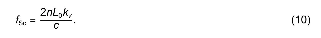

3.3.Multiplexed EFPIs


3.4.Resolution Limitations


3.5.Noise Compensations in a Pair of EFPIs
4.Experimental Demonstration
4.1.Single Air-Gap EFPI for Static Signals
4.2.Single EFPI,Wafer-Based for Static Signals
4.3.Single Air-Gap EFPI for Dynamic Signals

4.4.Multiplexed EFPIs with Static Perturbations

4.5.Temperature Measurement by Single and Multiplexed EFPIs
4.6.Resolution Improvement Be Means of Noise Compensations

5.Conclusion
 Journal of Electronic Science and Technology2020年1期