N-SOLITON SOLUTION OF THE KUNDU-TYPE EQUATION VIA RIEMANN-HILBERT APPROACH?

Lili WEN(溫麗麗)Ning ZHANG(張寧)Engui FAN(范恩貴)?

1.School of Mathematical Sciences,Fudan University,Shanghai 200433,China

2.Department of Basic Courses,Shandong University of Science and Technology,Taian 266510,China

E-mail:wenllerin@163.com;zhangningsdust@126.com;faneg@fudan.edu.cn

Abstract In this article,we focus on investigating the Kundu-type equation with zero boundary condition at in fi nity.Based on the analytical and symmetric properties of eigenfunctions and spectral matrix of its Lax pair,a Riemann-Hilbert problem for the initial value problem of the Kundu-type equation is constructed.Further through solving the regular and nonregular Riemann-Hilbert problem,a kind of general N-soliton solution of the Kundu-type equation are presented.As special cases of this result,the N-soliton solution of the Kaup-Newell equation,Chen-Lee-Liu equation,and Gerjikov-Ivanov equation can be obtained respectively by choosing different parameters.

Key words the Kundu-type equation;Lax pair;Riemann-Hilbert problem;soliton solution

1 Introduction

In this article,we will investigate the Kundu-type equation[1–3]

which can be used to describe the propagation of ultrashort femto-second pulses in an optical fi ber[4–6].In equation(1.1),u is the complex envelope of the wave,denotes its complex conjugate,the subscript denotes the partial derivative to the variables x and t.The N-soliton solution and high-order rogue wave solutions of equation(1.1)were obtained by Darboux transformation in[3,7].The Kundu equation was firstly obtained by Kundu in the studying of the gauge transformations for the nonlinear Schr?dinger-type equations[1,2].The equation(1.1)is related to three kinds of celebrated derivative nonlinear Schr?dinger equations.For β =0,equation(1.1)reduces to the Kaup-Newell equation which is called the first type of derivative nonlinear Schr?dinger equation[8–12]

Here we should point that there are some differences between the Kundu-type equation(1.1)and the following Kundu-Eckhaus equation

which was investigated via Darboux transformation method[20].First,the Kundu-type equation(1.1)is explicitly related to three derivative NLS equations(1.2)–(1.4);the Kundu-Eckhasu equation(1.5)can reduce to NLS equation(β=0),but not explicitly reduce to above three derivative NLS equations.Second,they have different spectral problems and Lax pairs,the Kundu-type equation(1.1)admits spectral problem

which is a generalization of KN spectral problem;while the Kundu-Eckhaus equation(1.5)has spectral problem

which a generalization of NLS spectral problem.

The inverse scattering transform is an important method to construct the exact solutions of completely integrable systems[21].The Riemann-Hilbert formulation is a new version of inverse scattering transform which was widely adopted to solve nonlinear integrable models[14,19,22–24,26–33].The purpose in this article is to construct the N-soliton solution for the equation(1.1)via the Riemann-Hilbert approach.

This article is organized as follows.In Section 2,starting from the Lax pair of the Kundu equation,we analyze the analytical and symmetric properties for eigenfunction and scattering matrix.In Section 3,we construct the Riemann-Hilbert problem and establish its connection with the solution of the Kundu equation.Section 4,we obtain the formal solutions for regular Riemann-Hilbert problem and the irregular Riemann-Hilbert problem,and obtain the N-soliton solution for equation(1.1).By taking different values for parameter β,we give the soliton solutions of the Kaup-Newell equation,Chen-Lee-Liu equation and Gerjikov-Ivanov equation,respectively.In Section 5,we summarize the results obtained in this article as a conclusion.

2 Spectral Analysis

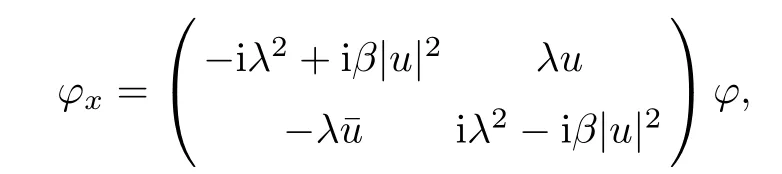
Equation(1.1)admits the following Lax pair

where

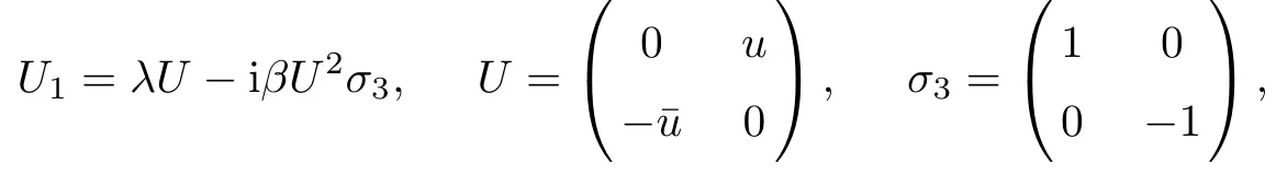
where λ is the spectral parameter.In analysis,we assume that initial value u(x,0)=u0(x)decays to zero sufficiently fast as|x|→∞.In this way the Lax pair(2.1)admits Jost solution with the following asymptotic

We make transformation

and change the Lax pair(2.1)into

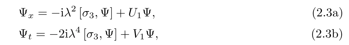
where[σ3,Ψ]= σ3Ψ?Ψσ3.

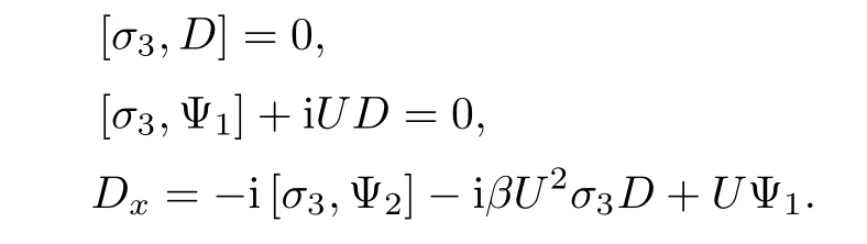
In order to formulate a Riemann-Hilbert problem for the solution of the initial value problem,we seek solutions of the spectral problem which approach the 2×2 identity matrix as λ→∞.For this purpose,we write the solution of the Lax pair(2.3)Ψ in the Laurent series as

where D,Ψn(n=1,2,···)are independent of λ.Substituting the above expansion(2.4)into(2.3a),and comparing the coefficients of λ,we obtain the following equations

In the same way,substituting expansion(2.4)into(2.9a),and comparing the coefficients of λ,we obtain the following equations

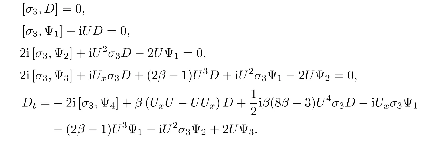
From these equations,we find D is a diagonal matrix and obtain the following equations

which implies that(2.5)and(2.6)for D are consistent,so that

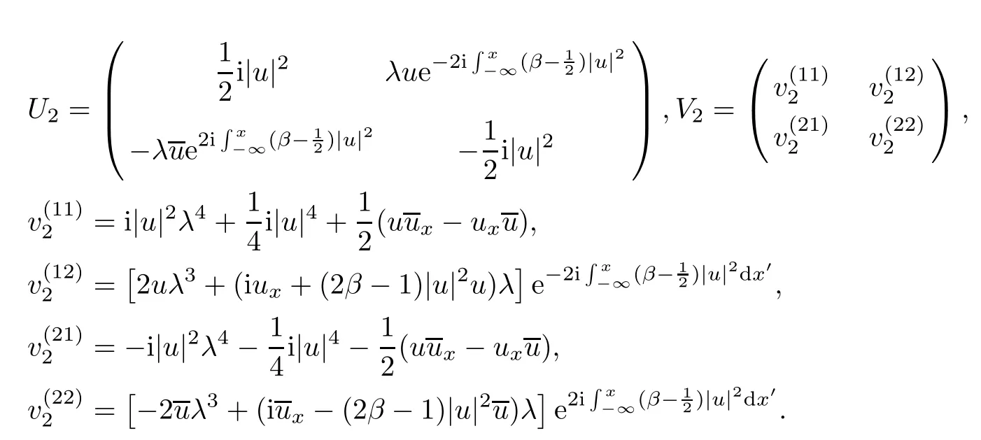
We introduce a new spectral functionμby

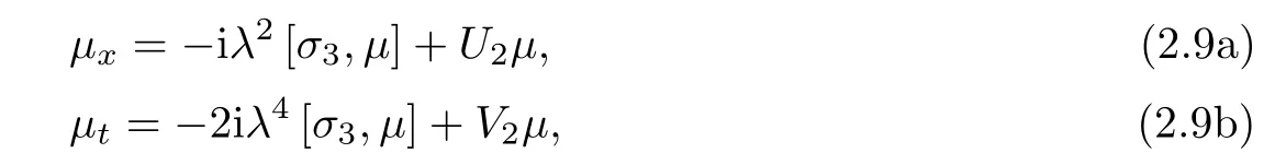
where

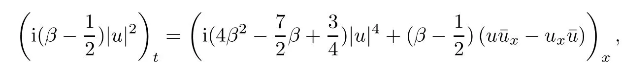
It is easily known that Lax pair(2.9)can be written in full derivative form

Also direct calculation from(2.7)and(2.8)shows that

We assume that u(x,t)is sufficiently smooth.Following the idea in[25],we can obtain the Volterra integral equations

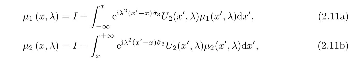
which meet the asymptotic condition

and we have

where I is the 2×2 identity matrix.

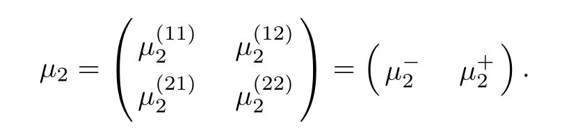
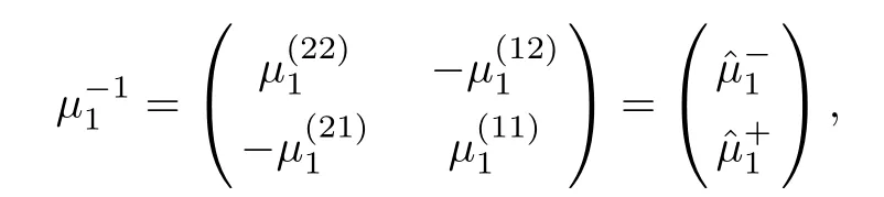
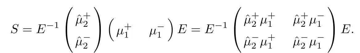
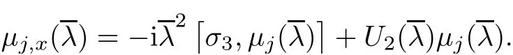
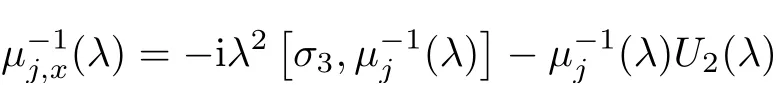
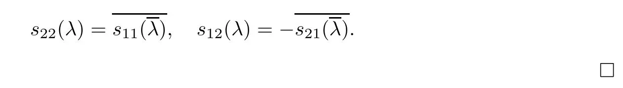
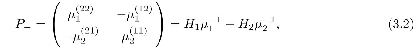
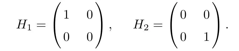
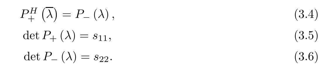
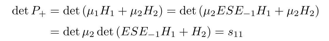
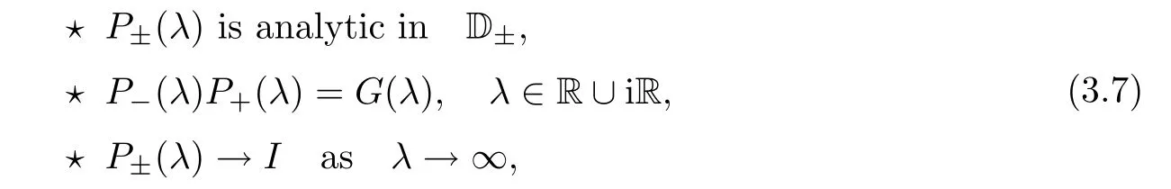
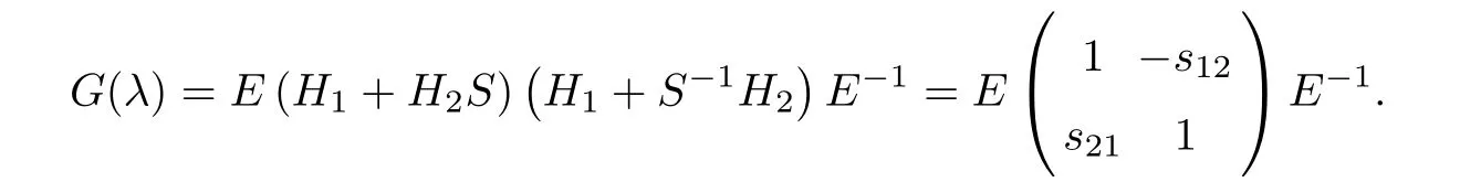
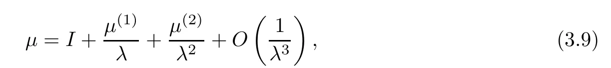
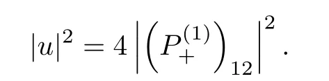
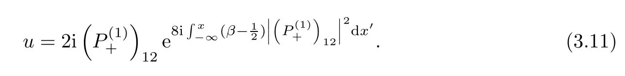
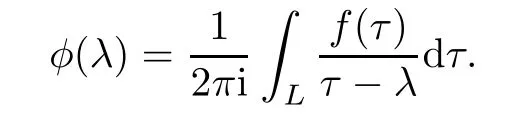
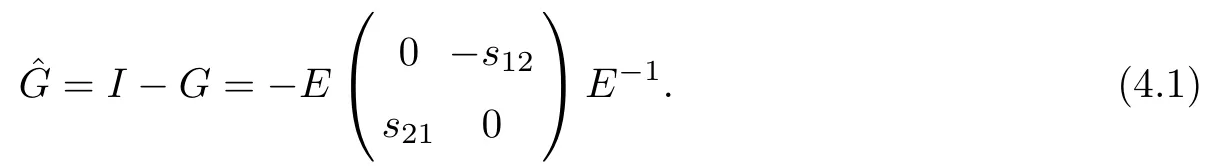
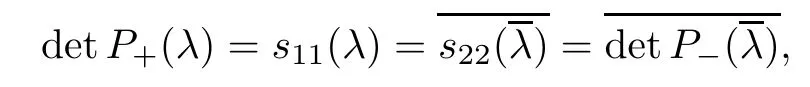
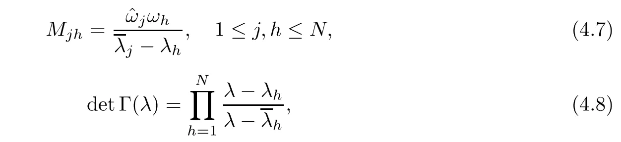
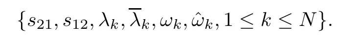
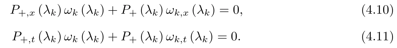
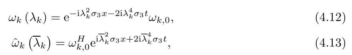
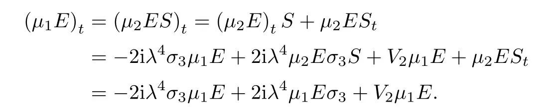
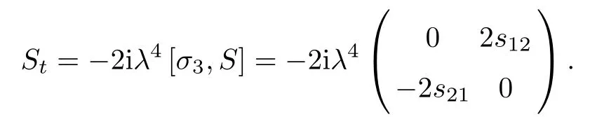
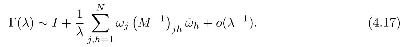
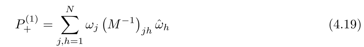
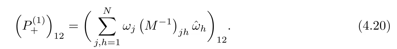
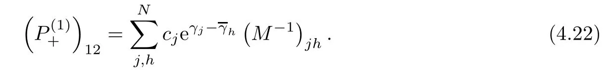
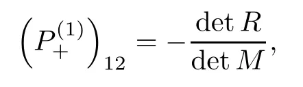
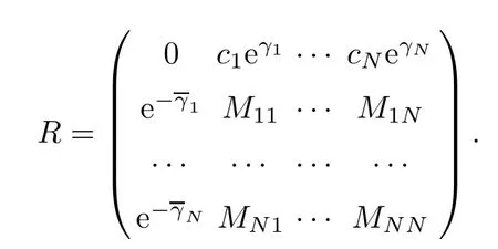
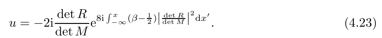
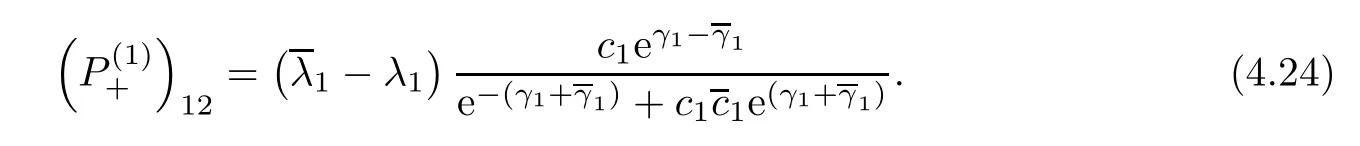
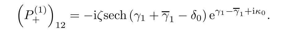
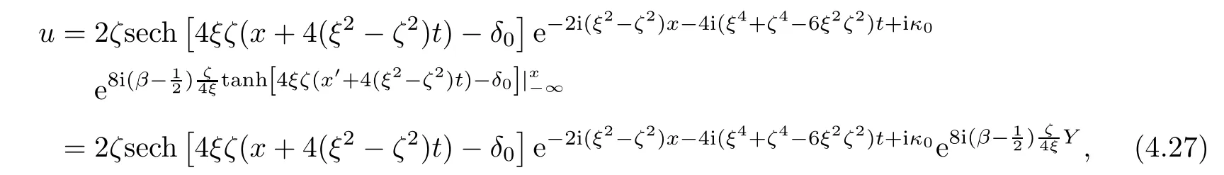
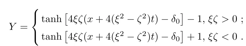
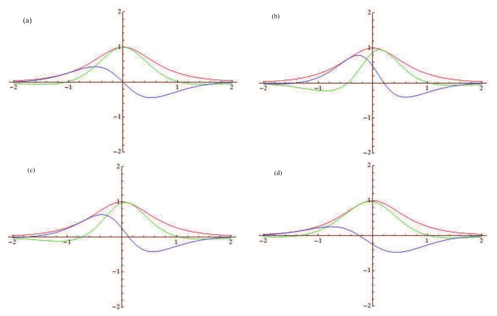
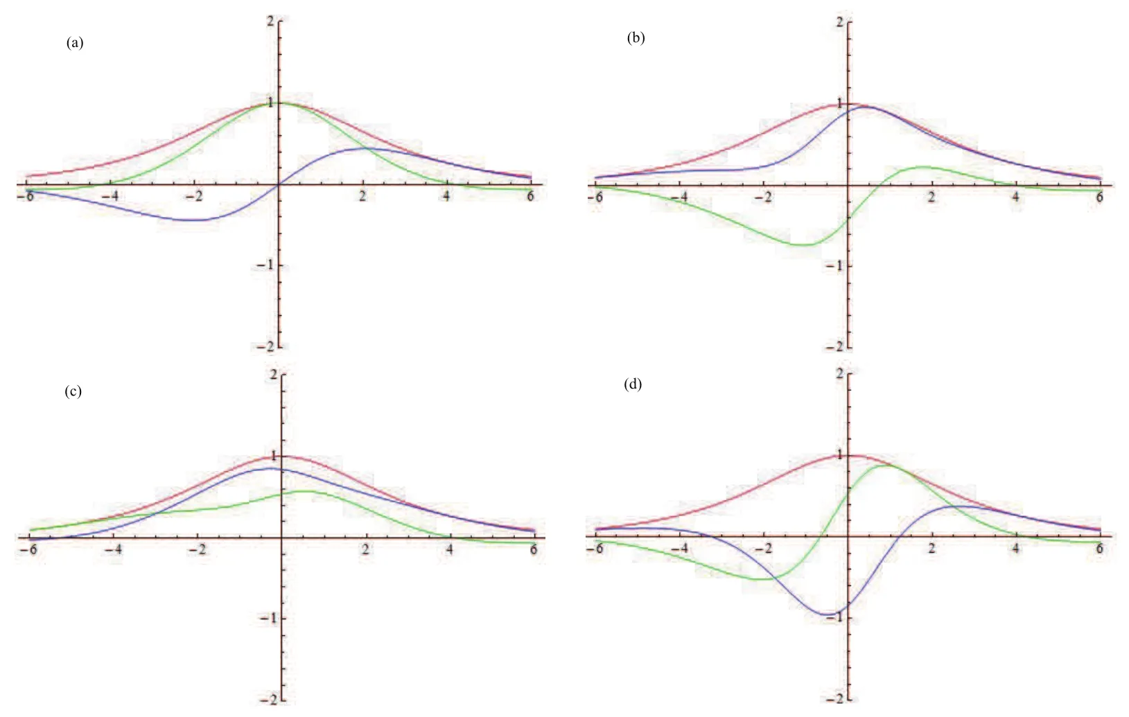
Forμ1,as x′

Then,the first column of and the second column ofμ1can be analytically extended to D+={λ |ReλImλ >0}and D?={λ |ReλImλ <0},respectively.We denote them in the form

where the superscript ‘±’refer to which half of the complex plane the vector function are analytic in,and

In the same way,the first column ofμ2and the second column ofμ2can be analytically extended to D?and D+,and we denote them in the form

Denote E=e?iλ2xσ3,then from relation(2.2),we know that ?1= Ψ1E and ?2= Ψ2E are both the solutions of the first order homogeneous linear differential equation(2.1).So they are linearly related by a matrix S(λ)=(sij)2×2,that is,

From Lax pair(2.1),we know that

Therefore,det?1,det?2are independent of x and t.Again by using relations(2.2)and(2.8),we can show that detμjis a constant.Making use of the asymptotic condition(2.12),we obtain

Taking determinant for the both sides of(2.14)gives

As a result of detμj=1,we note thatμjare invertible matrices.According the analyticity of the column vector functions ofμj,we known that the first row and the second row ofcan be analytically extended to D?and D+,

the first row and the second row ofcan be analytically extended to D?and D+

Thus,we have

It indicates that s11and s22are analytic in D+and D?,respectively,s12and s21do not analytical in D±,but continuous when λ∈ R∪iR.

Theorem 2.1The functions μj(λ),(j=1,2)and S(λ)satisfy the symmetry properties

where the superscript ‘H’denotes the conjugate transport of a matrix.

ProofReplacing λ byin(2.9a),

We see that

and have the asymptotic property

Then,we have the symmetry property(2.15).Expand equation(2.15),we have

In the same way,replacing λ byin(2.14),and we obtain

Substitute(2.15)into equation(2.18),we obtain symmetry property(2.16).Furthermore,we have

3 Riemann-Hilbert Problem

In this section,we introduce matrix Jost solutions P±according the analytic properties ofμj.Then,the Jost solution

which is an analytic function of λ in D+;and

which is an analytic function of λ in D?,where

In addition,

Theorem 3.1P±(λ)satisfy the following properties

ProofFrom properties(2.15)and(3.1),we obtain

Furthermore,we have the following equations

and in the same way,we have detP?(λ)=s22.

Summaring above results,we arrive at

where jump matrix is

We will turn to solve the Riemann-Hilbert problem.

We obtain a solution(2.4)of the Lax pair(2.3).If we expand P±and μ at large λ as

and using(2.10),(3.1),(3.2),(3.8),(3.9),we find that

and

Then we obtain

4 Solving the Riemann-Hilbert Problem

4.1 The Regular Riemann-Hilbert Problem

The regularity means that both detP±6=0 in their analytic domains.Under the canonical normalization condition,the solution to this regular Riemann-Hilbert problem is unique.However,its expression is not explicit,but the formal.

Theorem 4.1(Plemelj formula) Assume that L is a simple,smooth contour or a line dividing the complex λ plane into two regions ?+and ??,and f(τ)is a continuous function on the contour L.Suppose a function φ(λ)is sectionally analytic in ?+and ??,vanishing at in fi nity,and on L,φ+(λ)?φ?(λ)=f(λ), λ ∈ L,where φτis the limit of φ(λ)as λ approaches τ∈ L in Γ±.Then we have

To use the Plemelj formula on the regular Riemann-Hilbert problem,we need to rewrite equation(3.7)as

where

Applying the Plemelj formula to above equation and utilizing the boundary conditions,the unique solution of the regular Riemann-Hilbert problem can be presented by the following equation

4.2 The Non-Regular Riemann-Hilbert Problem

The irregularity means that detP±possess certain zeros at in their analytic domains.Then

this equation indicate that detP+(λ)and detP?(λ)with the same zeros number.We assume that detP+and detP?have N zeros λk∈ D+,and∈ D?,1 ≤ k ≤ N,where N is the number of zeros.Furthermore,we have the following relationdenotes the complex conjugation of λk.For simplicity,we assume that all zeros are simple zeros of detP±.At this point,the kernels of P+(λk)and P?contain only a single column vector ωkand row vector,i.e.,

By utilizing property(3.4),we find

Theorem 4.2(see[22]) The solution to the nonregular Riemann-Hilbert problem(3.7)with zeros(4.4)under the canonical normalization condition(3.3)is

where

M is an N×N matrix with its(j,h)-th elements given by

The solution of the nonregular Riemann-Hilbert problem(3.7)as given in Theorem 4.2,and the scattering data needed to solve this nonregular Riemann-Hilbert problem is

Taking the x-derivative and t-derivative to the equation P+(λk)ωk(λk)=0,we obtain

Substitute equation(3.1)into(4.10)and(4.11),we obtain

from which we obtain that

where ωk,0is a constant column vector.

Noticing that bothμ1E and μ2E satisfy the equation(2.9),by using the relation(2.14),we obtain

Furthermore,we obtain

Then,

where s12(0,0)and s121(0,0)are arbitrary constants.

According to the formal solution of regular Remann-Hilbert problem,the formal solution(4.9)can be presented as

Thus,as λ→ ∞,

and

And as λ → ∞,

Substituting asymptotic expansions(3.8),(4.16)and(4.17)into equation(4.5)and comparing the coefficient of λ?1yields

4.2.1 N-Soliton Solution

Now,we solve the Riemann-Hilbert(3.7)in re fl ectionless case when s21(0,0)=s12(0,0)=0,which leads to?G=0,then(4.18)is simpli fied as

and

Without loss of generality,we let ωk0=(ck,1)T,and introduce the notation

Then

Thus

And(4.22)can be rewritten as

where

So,we have

When N=1,we have

Letting

And insert them into(4.24),we obtain

Furthermore,

Hence the one-soliton solution(3.11)can be further written as

where

Thus ξζ>0 when λ ∈ D+.Furthermore,for ξ< ζ(see Figure 2),the one-soliton solution is right traveling wave,for ξ> ζ(see Figure 1),the one-soliton solution is left traveling wave,and for ξ= ζ(see Figure 3),the one-soliton solution is a stationary wave.

Figure 1 One-soliton solution u with the parameters as ξ=1,ζ=,δ0=0,κ0=0,and t=0.(a)β=,(b)β=0,(c)β=,and(d)β=.Red line absolute value of u,green line real part of u,yellow line imaginary part of u

Figure 2 One-soliton solution u with the parameters as ξ=,ζ=,δ0=0,κ0=0,and t=0.(a)β=,(b)β=0,(c)β=,and(d)β=.Red line absolute value of u,green line real part of u,yellow line imaginary part of u

Figure 3 One-soliton solution u with the parameters as ξ=1,ζ=1,δ0=0,κ0=0,and t=1.(a)β=,(b)β=0,(c)β=,and(d)β=.Red line absolute value of u,green line real part of u,yellow line imaginary part of u

5 Conclusion

In this article,we have considered the zero boundary problem at in fi nity for Kundu-type equation via the Riemann-Hilbert approach.By the analysis of the analytical and symmetric properties of eigenfunctions and spectral matrix,the Riemann-Hilbert problem for the Kundutype equation is constructed.Through solving the regular and nonregular Riemann-Hilbert problem,a kind of general N-soliton solution of the Kundu-type equation are presented.As special cases,the N-soliton solution of the Kaup-Newell equation,Chen-Lee-Liu equation,and Gerjikov-Ivanov equation can be obtained respectively by choosing different parameters.The above results can be extended to zero boundary problem for Kundu-type equation,which will be considered in our future work.