Reliability analysis of earth dams using direct coupling

A.T.Sir ,G.F.Np-Grí ,A.T.Bek ,M.M.Futi ,b

a Department of Civil Engineering,University of S?o Paulo,S?o Paulo,Brazil

b Research Group GeoInfraUSP,University of S?o Paulo,S?o Paulo,Brazil

c Instituto Tecnológico Vale,Ouro Preto,Minas Gerais,Brazil

Keywords:Earth dam Geotechnical parameters Reliability analysis Water level

A B S T R A C T Numerical methods are helpful for understanding the behaviors of geotechnical installations.However,the computational cost sometimes may become prohibitive when structural reliability analysis is performed,due to repetitive calls to the deterministic solver.In this paper,we show how accurate and efficient reliability analyses of geotechnical installations can be performed by directly coupling geotechnical software with a reliability solver.An earth dam is used as the study object under different operating conditions.The limit equilibrium method of Morgenstern-Price is used to calculate factors of safety and find the critical slip surface.The commercial software packages Seep/W and Slope/W are coupled with StRAnD structural reliability software.Reliability indices of critical probabilistic surfaces are evaluated by the first-and second-order structural reliability methods(FORM and SORM),as well as by importance sampling Monte Carlo(ISMC)simulation.By means of sensitivity analysis,the effective friction angle(φ＇)is found to be the most relevant uncertain geotechnical parameter for dam equilibrium.The correlations between different geotechnical properties are shown to be relevant in terms of equilibrium reliability indices.Finally,it is shown herein that a critical slip surface,identified in terms of the minimum factor of safety(FS),is not the critical surface in terms of the reliability index.

1. Introduction

The conventional approach for seepage and slope stability analyses of dams is to use deterministic soil properties to find deterministic factors of safety(FSs)(Fredlund and Krahn,1977;Griffiths and Lane,1999;Cheng,2003;Sarma and Tan,2006).On the last four decades,much work has been done to quantify the variability of soil properties(Phoon and Kulhawy,1999a,b;Phoon et al.,2006)to determine the reliability index(β)and the probability of failure(Pf)of slopes and embankments(Wu and Kraft,1970;Alonso,1976;Tang et al.,1976;Li and Lumb,1987;Christian et al.,1994;Lianget al.,1999;Duncan,2000;Bhattacharya et al.,2003;Yanmaz et al.,2005;Xue and Gavin, 2007; Ching et al., 2009; Sivakumar Babu and Srivastava,2010;Calamak and Yanmaz,2014;Yi et al.,2015;Guo et al.,2018;Mouyeaux et al.,2018).

Probabilistic slope and dam stability analyses can be performed using different approaches.Monte Carlo simulation(MCS)is by far the most intuitive and well-known probabilistic method;however,it usually implies a very large computational burden.Point estimate methods (PEMs) are popular in geotechnical engineering(Rosenblueth,1975;Hong,1998;Zhao and Ono,2000),but they are inaccurate for many problems(Napa-García et al.,2017).Using higher-order moment methods increases computation accuracy,but the efficiency is lost.Transformation schemes such as first-and second-order reliability methods(FORM and SORM)are competitive with PEMs,in terms of computational effort,but are more appropriate and accurate for evaluating small failure probabilities controlled by distribution tails.The FORM loses accuracy when dealing with highly nonlinear limit state functions,where PEMs also fail.

One particularity of reliability analysis for stability of slopes and dams is the location of the critical slip surface,which is critical for safety control.A dam or slope may fail at a circular or non-circular slip surface,but during the mathematical procedure,an infinite number of slip surfaces are tested.Evaluating the total failure probability along all potential slip surfaces is considered as a mathematically formidable task(El-Ramly et al.,2002).It has been shown that the surface of the minimum FS is not always the surface of the maximum probability of failure(Hassan and Wolff,1999); hence, a probabilistic search for the critical surface is required.Dam or slope reliability is often determined only for one or a limited number of slip surfaces(Tang et al.,1976;Hassan and Wolff,1999; El-Ramly et al., 2002; Wang et al., 2011). It is generally recognized that search for the critical probabilistic slip surface is similar, in principle, to that for the surface of the minimum FS in the deterministic approach(Cheng et al.,2015).Low et al.(1998)developed a spreadsheet procedure for evaluating the reliability of slopes using the method of slices.The procedure is easy to follow,but it is limited to simple geometries,uniform geotechnical properties and Gaussian random variables.In contrast,the direct coupling method explored herein can be applied to complex geometries,nonlinear geotechnical analysis,arbitrary probability distributions and nonuniform pore pressure and strength profiles.

Some commercial software packages,such as Slope/W(Geo-Studio)and Slide(RocScience),perform slope stability analysis probabilistically using MCS and the following second-moment approximation (Baecher and Christian, 2003; Phoon, 2008;Duncan et al.,2014;Phoon and Ching,2015):

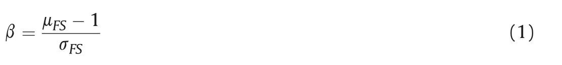
where μFSis the mean value and σFSis the standard deviation of the trial FS.These programs have some limitations in terms of statistical distributions of hydraulic or mechanical properties,as well as for specific structural reliability methods,such as FORM and SORM.

Other programs have been developed to integrate slope stability and reliability analyses,such as 3DSTAB(Yi et al.,2015)and SCU-SLIDE(Wu et al.,2013),which use MCS to evaluate the reliability index in Eq.(1).In contrast to the above references and approaches,the so-called direct coupling(DC)technique(Sudret and Der Kiureghian, 2000; Leonel et al., 2011; Napa-García,2014;Kroetz et al.,2018;Mouyeaux et al.,2018)appears to be an efficient method for finding the critical probabilistic slip surface and evaluating structural reliability in slope and dam stability problems.

In this paper,the DC technique is employed to combine the deterministic software GeoStudio 2018 (GeoStudio, 2018a, b)with the structural reliability program StRAnD 1.07(Beck,2008).In this technique,the StRAnD software establishes the values of the random geotechnical parameters that the deterministic GeoStudio solution needs to be computed.StRAnD follows the FORM,SORM or MCS algorithms,as required by the user,and computes the failure probabilities.Gradients of the limit state function,required in the FORM and SORM,are evaluated by finite differences.The nomenclature DC is not evident in the literature, because in structural analysis, for instance, this approach is the rule, with other techniques being employed eventually(Kroetz et al.,2018).In this paper,application of the DC technique to a case study involving a dam is shown in a step-by-step fashion.

The coupled StRAnD-GeoStudio software is employed in Siacara et al.(2020)in the rapid drawdown analysis of earth dams;hence,the work in Siacara et al. (2020) presents application of the methodology presented herein,to a more specific problem.Under rapid drawdown conditions,the importance of the random seepage analysis for pore pressure variations increases.

2. Problem setting

A common approach to perform probabilistic analysis of slope stability is to identify the critical surface to obtain the minimum FS and then calculate the probability of failure for this surface.However,the surface of the minimum FS may not be the surface of the maximum probability of failure(Hassan and Wolff,1999).This problem has been addressed in a number of recent publications(Hassan and Wolff,1999;Li and Cheung,2001;Bhattacharya et al.,2003;Sarma and Tan,2006;Cheng et al.,2015;Reale et al.,2016).

2.1. Performance function

A structural reliability problem is formulated in terms of a random variable vector,X={X1,X2,…,Xn},representing a set of random geotechnical parameters.A performance function g(X)is formulated in such a way that x|g(x)≤0 is the failure domain,where x is a realization of X.In an“n”dimensional hyper-space of variables,the limit state function g(x)=0 is the boundary between safe and failure domains.The probability of failure is given by

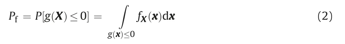
where fX(x)represents the joint probability density function of x.In numerical slope stability problems,the integral in Eq.(2)can be difficult to evaluate,as the limit state function is not given in analytical form;hence the integration domain is not given in closed form.In these cases,it is common to make a transformation y=T(x)to the standard Gaussian space;the minimum distance of the limit state function g(y)=0 to the origin is the so-called reliability index(β),and the point over the limit state with minimum distance to the origin is called the“design point”.In the standard Gaussian space,the limit state function is approximated by a hyperplane,yielding the classic first-order approximation:

where φ(?) is the standard Gaussian cumulative distribution function(Melchers and Beck,2018).

In slope stability problems,the performance function can be written as(Phoon,2008):

The Morgenstern-Price stability analysis method is employed herein to evaluate FS.The critical surface is calculated for each realization of X in search of the design point.Hence,although the critical surface is not given explicitly in terms of a particular random variable,the most probable critical surface is found.

2.2. Finite difference evaluation of performance function gradients

The search for the design point in transformed y space using mathematical programming techniques involves evaluation of the gradient of the limit state function with respect to the vector of random variables:

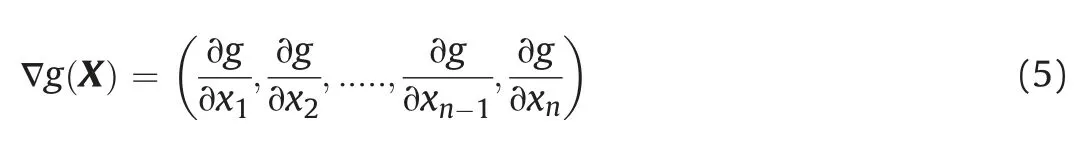
Progressive, regressive or central finite differences can be employed to evaluate this gradient numerically.In progressive finite differences employed herein,each component of ?g(?)requires one computation of the numerical response:

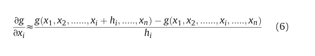
where hiis the step size or increment.In the first iteration,the step size is given as a fraction of the standard deviation of each random variable:

where fstepis the fraction of the standard deviation σXiused as step size.

From the second iteration onwards,the step is given as a fraction of the change in x from the past iteration:

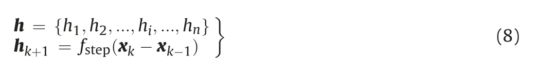
A minimum value of hminis used to avoid numerical instability in computations.The optimal size of fstepcan be found by minimizing the differentiation and numerical errors of the approximation(Gill et al.,1981;Scolnik and Gambini,2001).

Each evaluation of the gradient vector requires“n+1”solutions of the numerical model.The limit state responses in Eq.(6)are evaluated directly by calling the numerical solver from the structural reliability software StRAnD 1.07(Beck,2008).This approach is known as DC in the literature(Sudret and Der Kiureghian,2000;Leonel et al.,2011;Napa-García,2014;Kroetz et al.,2018).If the numerical algorithm used to find the design point requires m iterations to converge,the total number of limit state function calls is m(n+1).As observed by Leonel et al.(2011),such a solution is more economical than constructing adaptive surrogate models for the limit state function,a popular approach in geotechnical reliability analyses.

2.3. The first-order reliability method(FORM)

As mentioned previously,the FORM consists of mapping the problem from the original design space X to the standard Gaussian space Y by means of a transformation y=T(x),where y is a realization of Gaussian vector Y.This transformation can deal with non-Gaussian variables as well as the correlation between random variables(see Fig.1).The transformation is accomplished by means of the principle of normal tail approximation(Ditlevsen,1981;Der Kiureghian and Liu,1986)and the Nataf model(Nataf,1962),following the work of Melchers and Beck(2018).

In standard Gaussian space,the so-called design point is found by solving the following constrained optimization problem:Find y*which minimizes yTy,subjected to g(y)=0.

The solution of this problem requires iterative procedures due to general nonlinearity of the limit state function and the nonlinearity of y=T(x)mapping.The point y*is found as the solution to the constrained optimization problem is also known as the design point among all points in the failure domain,and it is the point most likely to occur.Hence,this point corresponds to the most likely combination of geotechnical parameters,leading to loss of equilibrium.The critical slip surface is found in each iteration,and the critical surface most likely to occur is at the end of the iterative procedure,herein it is called the probabilistic slip surface.

At the design point,the original limit state function is replaced by a hyper-plane:the failure probability becomes the probability mass beyond the hyper-plane.The Hasofer-Lind reliability index is given by β=[(y*)T(y*)]1/2,and the failure probability estimate is given by Eq.(3).The accuracy of the FORM approximation depends on the degree of nonlinearity of the limit state in Y space.The solution is exact only for linear functions of independent Gaussian random variables(Melchers and Beck,2018).For nonlinear limit state functions,improved estimates of the failure probability are obtained by replacing the hyper-plane by a quadratic or parabolic hyper-surface,at the design point.This requires evaluating the curvatures of the limit state function at the design point and is known as SORM (Fiessler et al., 1979; Breitung, 1984; Der Kiureghian et al.,1987;Tvedt,1990).

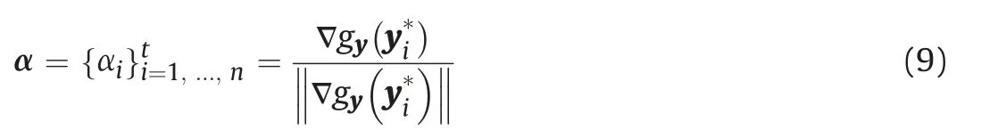
Important sub-products of the FORM solution are the so-called sensitivity factors,which are obtained from

2.4. “Crude”Monte Carlo simulation(MCS)

The probability of failure(Pf)in Eq.(2)can also be evaluated directly by means of“crude”MCS.By employing an indicator function I(x),the integration in Eq.(2)can be extended over the whole domain,based on samples generated from fX(x):

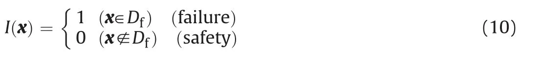
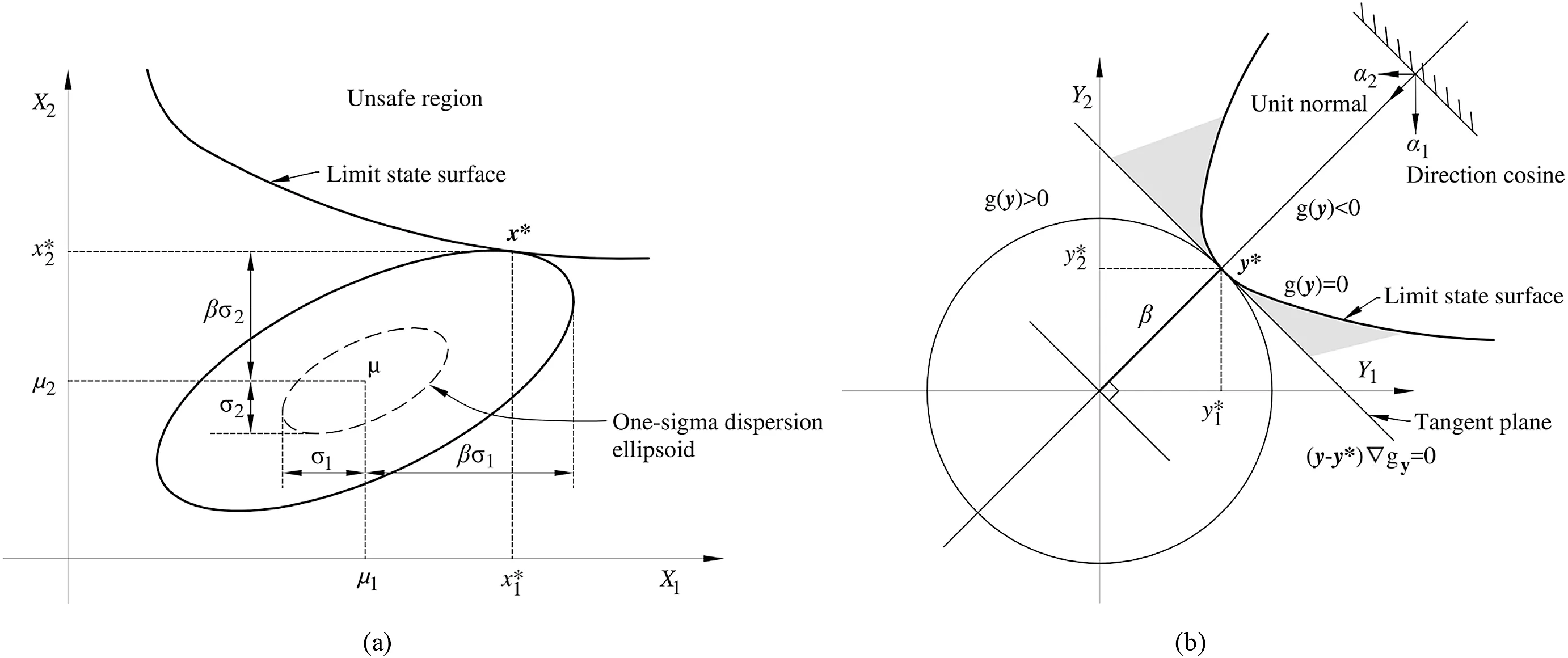
Fig.1.FORM transformation from(a)original(X)to(b)standard Gaussian(Y)space(based on Ji et al.,2018;Melchers and Beck,2018).

Therefore,the expected value of the probability of failure can be estimated,based on a sample of finite size,by

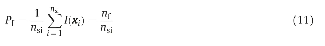
where nfis the number of points in the failure domain and nsiis the number of simulations.The mean in Eq.(11)is a unbiased estimator of the probability of failure:the estimate converges to the exact probability of failure in the limit,as nsi→+∞.

2.5. Importance sampling Monte Carlo(ISMC)simulation

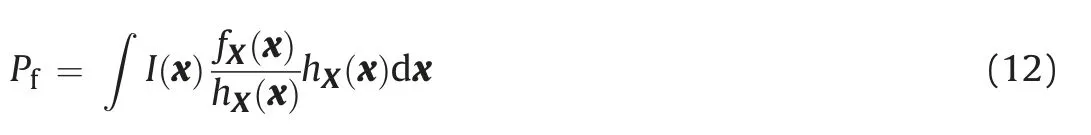
Importance sampling using design points concentrates sampling points at important regions of the failure domain.This technique reduces the number of simulations by avoiding excessive simulation of points away from the region of interest,i.e.away from the failure domain.These techniques generally make use of additional information about the problem,such as the coordinates of the design point.A strictly positive sampling function hX(x)is employed to generate the samples;this function is centered at the design point:

The weight corresponding to each sample is

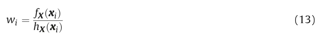
The mean probability of failure,for a sample of size nsi,becomes

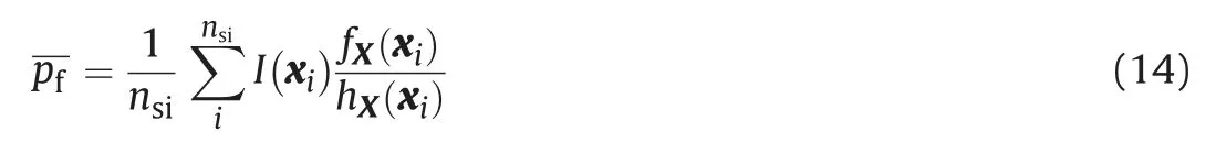
The solution is subjected to a sampling error or variance,which is estimated by

From Eqs.(14)and(15),the confidence interval(CI)of MCS is estimated as

where parameter k is related to the desired confidence(Beck,2019).

3. Methodology

3.1. Steps of the probabilistic modeling

The numerical calculations were implemented by coupling GeoStudio 2018(GeoStudio,2018a,b)and StRAnD 1.07(Beck,2008)software.The coupled program can be used to evaluate the safety and structural reliability of earth dams in different conditions and other structures from this developed methodology.Using a deterministic approach and different limit equilibrium methods(LEMs)(e.g.Morgenstern-Price),FSs are evaluated.Using the structural reliability methods presented herein(e.g.FORM,SORM and ISMC),the reliability index(β)and corresponding probabilities of failure(Pf)are evaluated.

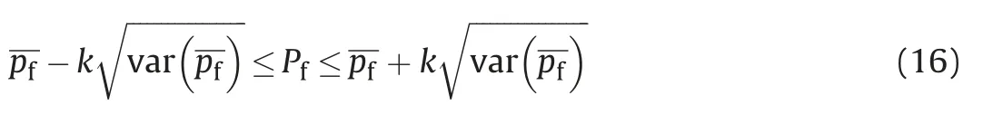
This section presents an overview of the procedure implemented to evaluate the reliability of earth dams based on coupling deterministic software(GeoStudio,2018)with structural reliability software(StRAnD 1.07).The following procedure is illustrated by the flowchart in Fig.2:

(1)Initial information:Basic studies(e.g.topography,hydrology and geology),previous studies,standard tests,etc.

(2)Define the deterministic model:Choose and set up a twodimensional(2D)model(unique option in GeoStudio 2018 software).There are two steps to perform a deterministic analysis.First,seepage analysis is performed in Seep/W.Next,the LEM is performed using the pore water pressure of the previous step in Slope/W. The seepage analysis contains the representation of the soil-water characteristic curve(SWCC)and the hydraulic conductivity function;the LEM evaluates the shear failure of the slope for unsaturated soils.

(3)Define deterministic (nominal) data for geomaterial properties.

(4)Define the probabilistic model:Choose reliability methods in StRAnD 1.07 software.The reliability methods and conditions of correlation materials are defined in the STRAND_INPUT.txt file of the StRAnD software.

(5)Define probabilistic data for geomaterial properties.

(6)Master program:All deterministic and probabilistic analyses presented in the flowchart(Fig.2)are performed using Visual Studio 2017 software compiler.

(7)Characteristic of FORTRAM code:The GeoStudio 2018 file contains the Seep/W and Slope/W information.The file has a format“.gsz”which is a ZIP file.The file is compressed/uncompressed from the 7-zip software saving the FS to find the design point(DP).All input parameters are changed in the file extension“.xml”,which is changed in every simulation or during a search for the DP).In the same folder,all the output data are found in the file extension“.csv”,which are used as the input parameters for the reliability analysis.

(8)The results of the reliability analysis(number of evaluations and simulations,sensitivity coefficients at DP,reliability index,probability of failure,evaluation time,DP,etc.)are shown in the STRAND_OUTPUT.txt file.In the GeoStudio software,all the critical slip surfaces for every simulation or at the DP are shown.

(9)Changes in the model:The deterministic methods,geometry and load conditions are changed in the GeoStudio software.The reliability methods and conditions are changed in the STRAND_INPUT.txt file of the StRAnD software.All changes in the GeoStudio file produce slight modifications in the FORTRAN code,whereas changes in the reliability analysis need no modifications in the FORTRAN code.

3.2. The application problem and boundary conditions

An earth dam was used as an example to test the performance of DC in three different operating cases(OPCs)for a long-term steadystate analysis.

The dam in this study consists of an earth embankment with 20 m height and 7 m width at the crest.In addition,the dam body was considered homogeneous with its different elements.The dam has a horizontal filter(approximately 2 m depth)to reduce pore pressure within the dam,conducting the water downstream.The upstream and downstream side slopes are 1V:3H(relation in meters of one vertical to three horizontal),and downstream of the dam is a berm with 3 m width.The freeboard is considered to be 3 m under the crest of the dam, and the outlet works are considered to be 3 m above the rock foundation;the maximum water level(W.L.MAX.)is 17 m,and the minimum water level(W.L.MIN.)is 3 m.The dam foundation is located in unweathered rock.

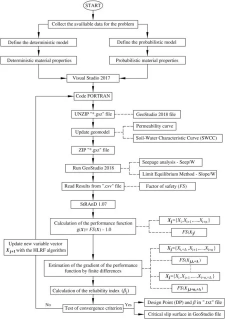
Fig.2.Flowchart of using StRAnD-GeoInfraUSP for the reliability analysis procedure by coupling GeoStudio and StRAnD software.

Fig.3.Critical cross-section of the dam.

Three OPCs of water level(W.L.)are studied,measured from the top of the unweathered rock:Case OPC 1 is the minimum,with a water level 3 m above the unweathered rock;Case OPC 2 has awater level 10 m above;and Case OPC 3 has a water level of 17 m,3 m below the crest.The saturated-unsaturated seepage and the stability of the slopes in the dam,considering the variability in the soil parameters,are studied herein.The main cross-section of the structure is shown in Fig.3.

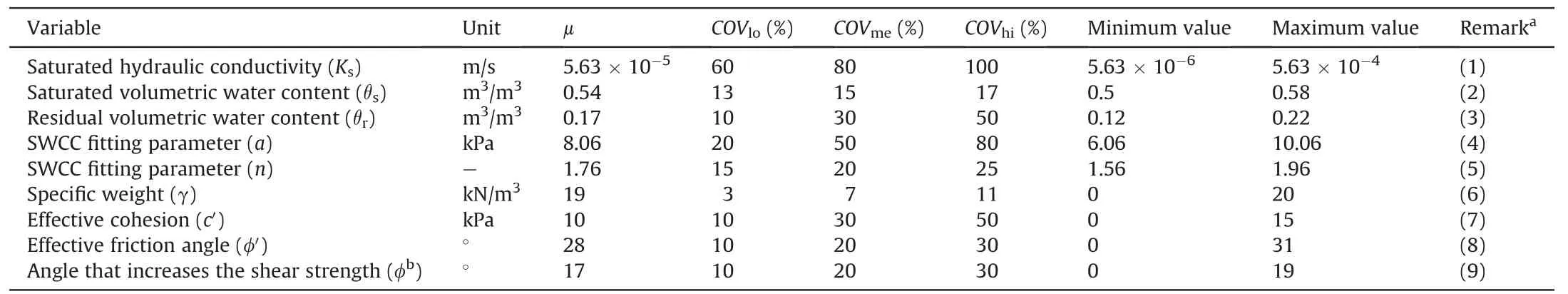
Table 1 Input soil parameters of the application problem.

Initially,the soil in the embankment is saturated under and unsaturated above the water table.The initial hydrostatic water pressure is given by the considered water level for each case of study,with positive pressure under and negative pressure above the water table.The water head on the upstream boundary beneath the water table is fixed,and the soil above the water table is permeable.The downstream boundary is treated as a seepage boundary. The bottom boundary is impervious (bedrock is considered waterproof and impenetrable).The upstream boundary condition is a constant 17 m of head for OPC 3 with the W.L.MAX.,10 m for OPC 2 in an intermediate condition,and 3 m for OPC 1 with the W.L.MIN.,whereas the downstream boundary condition is zero head.

The seepage analysis contains the representation of the SWCC and the hydraulic conductivity function predicted by using the van Genuchten equation(Van Genuchten,1980),and the Morgenstern-Price method(Morgenstern and Price,1965,1967)with the shear strength criteria of unsaturated soils(Fredlund et al.,1978)is used as LEM.

The hydraulic and strength mean parameters and their statistics of the lean clay(CL in the Unified Soil Classification System)are obtained from related studies in the literature,as shown in Table 1.The random seepage analysis is characterized by the uncertainty of two SWCC fitting parameters(a and n),the saturated and residual volumetric water contents(θsand θr),and the saturated hydraulic conductivity parameter(Ks).The random stability analysis is characterized by uncertain specific weight(γ),effective cohesion(c＇),effective friction angle(φ＇),and the angle that increases shear strength(φb).The uncertain parameters of the stability and seepage analyses are assumed to have normal(N),lognormal(LN)or truncated normal(TN)distributions in the three different case studies.The mean(μ)and the coefficient of variation(COV)of all parameters are shown in Table 1.

Compacted lean clay(CL)was considered;the nominal seepage parameters were based on Cuceoglu (2016), and the nominal properties involved in the stability calculation were taken from USBR(1987)and Fredlund et al.(2012).

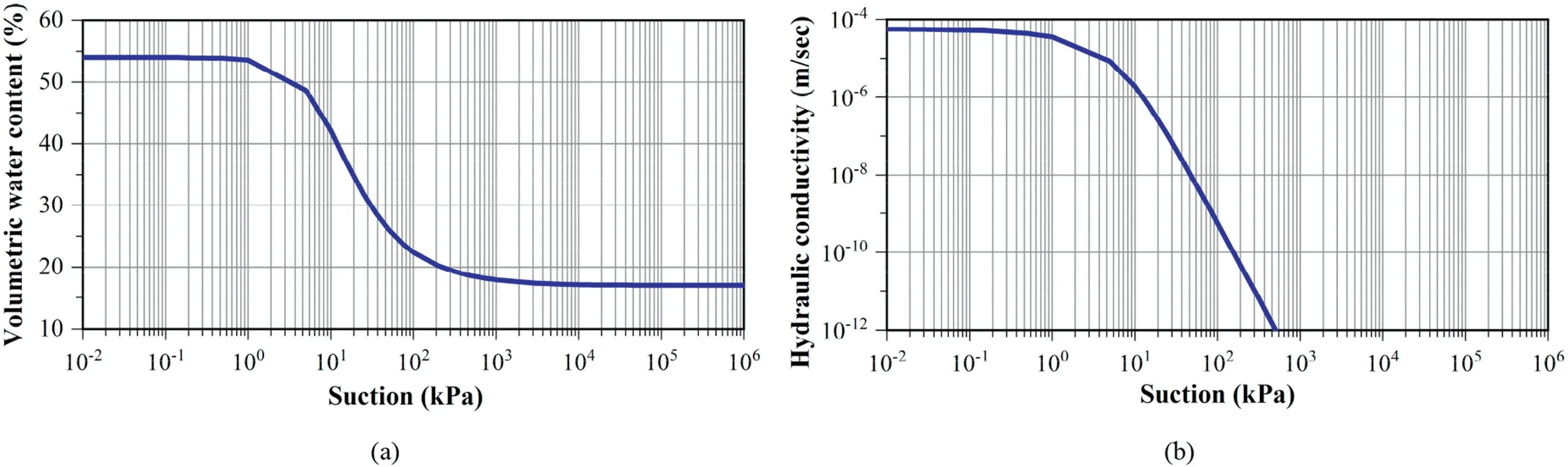
Fig.4.Mean values of hydraulic parameters:(a)SWCC and(b)Hydraulic conductivity curve.

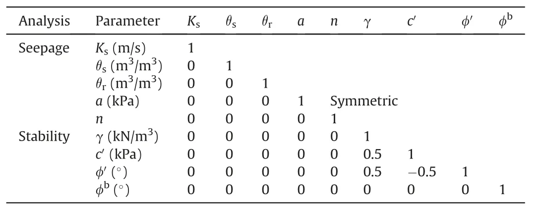
Table 2 Correlation coefficient matrix(ρ)between seepage and stability soil properties.

Large ranges of values from the minimum values to the maximum values of soil parameters were assumed to test the DC methodology in different operating conditions(Table 1).As shown in Table 1,the minimum values of soil parameters are taken as zero or a small positive number; this approach is appropriate for geotechnical parameters and avoids problems in the numerical computations.Minimum values are enforced in reliability analysis by choosing LN or TN distribution. Minimum values are not respected when geotechnical parameters are modeled using N distribution.The maximum values in Table 1 correspond only to the TN distribution from the largest value of a material property found in the literature;in addition,these values were assumed.Maximum values are not respected when geotechnical parameters are modeled using N and LN distributions.

Observing the COV values of hydraulic properties,the variability in the SWCC parameter n is smaller than that of parameter a;the variability in parameter θris smaller than that of parameter θs;and the COV of the saturated hydraulic conductivity ksis relatively large.Observing the COV values of the parameters involved in the stability calculation,it is verified that the variability in parameter γ is smaller than that of c＇and φ＇;and the variability in parameter φbis the same as that of φ＇.

For the mean values listed in Table 1,the corresponding SWCC and hydraulic conductivity curves are shown in Fig.4a and b,respectively.

In terms of COV values,three sets of soil property variabilities(low,medium and high)were employed,following Phoon(2008).These three sets of COV values depend on the level of uncertainty of these materials and on the quality of laboratory or field measurements.A low coefficient of variation(COVlo)is considered corresponding to good quality laboratory or field measurements;a medium coefficient of variation(COVme)is considered for indirect correlations with good field data,with the exception of the standard penetration test(SPT);and a high coefficient of variation(COVhi)is considered for indirect correlations with SPT field data and with strictly empirical correlations.

The correlation coefficient(ρ)is a dimensionless quantity that measures the linear dependency between pairs of random parameters.If the points in the joint probability distribution of two variables X and Y tend to fall along a line of positive slope,linear correlation between the variables exists,and the correlation is positive.If the slope is negative,so is the correlation.Positive or negative correlations imply linear dependency between the variables.If the variables are independent,the correlation is zero; however, zero correlation does not imply independency.

The correlation matrix ρ between the seepage and stability soil properties of the dam,as considered in this paper,is shown in Table 2.The correlation values are taken from the literature:the correlation between c＇and γ varies from 0.2 to 0.7;that between φ＇and γ varies from 0.2 to 0.7;and that between c＇and φ＇varies from-0.2 to-0.7,following Sivakumar Babu and Srivastava(2007),Wu(2013),and Javankhoshdel and Bathurst(2016).

3.3. Initial mean value analysis

The seepage and stability analyses were performed in the GeoStudio program(Seep/W and Slope/W)for three OPCs of the water level to obtain a deterministic(mean value)result for the most critical surface and for the FS.The mean value(μ)of the seepage properties(Ks,θs,θr,a and n)and properties involved in stability calculation(γ,c＇,φ＇and φb),presented in Table 1,were used in this analysis.A 2D analysis was performed in this paper.

Regarding the seepage analysis,a finite element analysis was performed for an earth dam to calculate pore water pressures.The finite element seepage analyses were also used to determine the position of the phreatic surface,which was plotted on the crosssection(e.g.the pore water pressure and the water total head from the OPC 3 analysis are shown in Fig.5).The phreatic surface was assumed to be the line of zero pore water pressure determined from the seepage analysis,as shown in Fig.5.

The pore water pressure and total water head for OPC 3 are shown in Fig.5.The pore water pressures were negative in the uppermost part of the flow region,above the phreatic surface.Negative pore water pressures were considered in the dam stability calculation.Negative pore water pressures had a minor contribution to dam stability,yet their effect was considered in this study.

Dam stability calculations were performed on the downstream slope using the pore water pressures obtained in seepage analysis.Morgenstern-Price procedure(Morgenstern and Price,1965,1967)was used for all calculations.To locate the critical slip surface for every representation of pore water pressure and OPC,an automatic search was performed by the entry(crest of the dam)and exit(toe of the dam)specification.The discretization for the entry and exit slip surface option was considered at every 0.1 m,and the circles were defined by specifying radius tangent lines.The critical surface of failure and the minimum FSs were determined using Slope/W;the results for OPC 3 are shown in Fig.6.This figure also shows the finite element mesh used to determine pore pressures in seepage analysis.

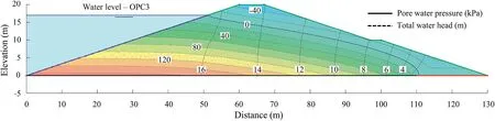
Fig.5.Results of the seepage analysis for OPC 3 with the pore water pressure(kPa)and total water head(m).

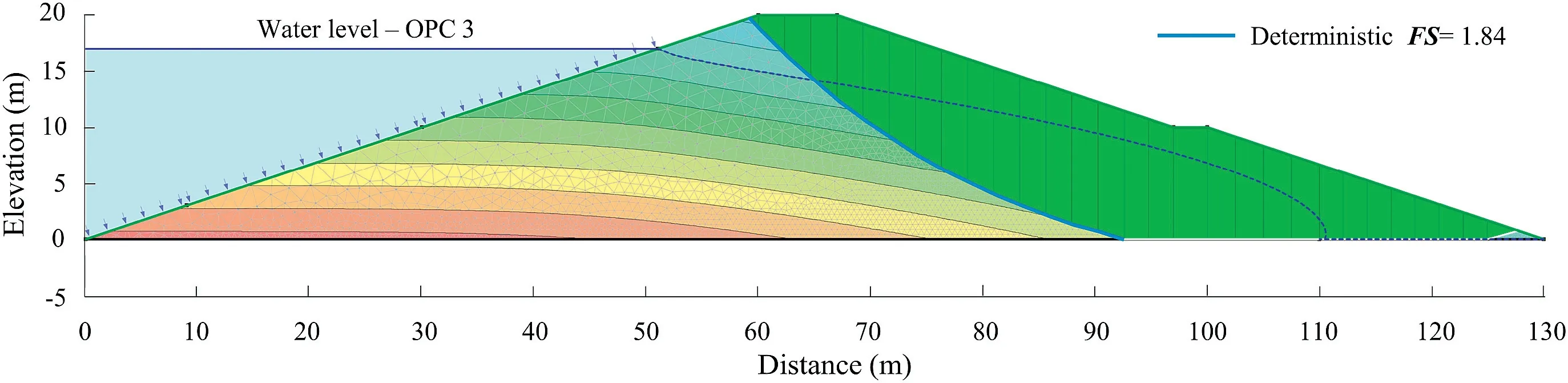
Fig.6.Critical surface for OPC 3.

Limit equilibrium analysis for the three OPCs resulted in different most critical surfaces and different FSs. During the seepage analysis,this analysis applies a phreatic surface adjustment with the interpolated pore water pressures of the finite elements.

In Slope/W software,all the slip surfaces must be contained in the domain of the model. The slip surface follows the boundary of the model when a trial slip surface intersects the lower boundary.Once a slip surface is generated,the portion of the slip surface that follows the lower boundary takes on the soil strength of the materials overlying the base of individual slices.This can always be verified by graphing the strength along the slip surface.It is just a mechanism to control the shape of trial slip surfaces.

From the stability analysis,a lower FS value of 1.84 was found for OPC 3,an intermediate value of FS=2.31 was found for OPC 2,and FS=2.64 was found for OPC 1.Clearly,the results show smaller FSs for higher water levels.The effect of φbincreases FS more in OPC 1 than in others.

The filter at the dam toe helps increase FS,reducing pore pressures in the dam.The Bureau of Reclamation(USBR,1987),US Army Corps of Engineers Slope Stability Manual(US Army Corps of Engineers,2003)and others(Duncan et al.,2014;Fell et al.,2015)recommended a minimum FS=1.5 for long-term steady-state seepage analysis of earth dams.All FSs evaluated herein in the mean value(deterministic)analysis satisfy this minimum stability criterion.

FSs provide a quantitative indication of dam stability for different water levels.A value of FS=1 would indicate a dam that is on the limit between stability and instability.If the values of the geotechnical parameters were perfectly known and if calculation models were perfectly precise,an FS of 1.1,or even 1.01,would be sufficient to warrant equilibrium. However, uncertainty about geotechnical parameters and imprecision of engineering models make larger FS be necessary(Duncan et al.,2014).Most often,recommended values for FS are determined based on previous experiences with similar structures,environments and calculation models.Structural reliability measures,such as the reliability index(β)or the probability of failure(Pf),can further inform whether a given dam structure is safe or not.Reliability measures are more complete in the sense that more information about the problem is explicitly incorporated in the analysis,such as standard deviation(or COV values)and the probability distribution of geotechnical parameters.

4. Reliability analyses and results

The results described herein were obtained using DC of GeoStudio and StRAnD software to find the reliability index(β)and the probability of failure(Pf),as described in Sections 2 and 3.Different sets of random material properties are considered,all taken from Tables 1 and 2 The initial analysis considers the whole set of nine random variables:five seepage random variables(Ks,θs,θr,a and n)and four stability random variables(γ,c＇,φ＇and φb).After sensitivity analysis is performed,some random variables with smaller contributions to failure probabilities are removed (or considered deterministic at mean values). The initial analysis considers the median values for coefficients of variation(COVme).

The following reliability analyses are presented in sequence:

(1)Initial results showing accuracy and differences in computational cost of FORM and SORM solutions,in comparison to ISMC;

(2)Sensitivity of the random variables, revealing the most important geotechnical parameters;only the most important random variables are considered in the rest of the analyses;

(3)Influence of the water level on the reliability indices;

(4)Influence of statistical distributions,comparing N,TN and LN distributions for all geotechnical parameters;

(5)Influence of the coefficients of variation(COVlo,COVme or COVhi)on the reliability indices;

(6)Influence of correlation(ρ)between material properties;and

(7)Comparison of critical slip surfaces found in deterministic and probabilistic analyses.

The limit state gradients are estimated using finite differences.The search for DP is performed with the Hasofer-Lind-Rackwitz-Fiessler (HLRF) algorithm for FORM and SORM. Finally, ISMC simulation is performed,with 1000 realizations.

4.1. Initial results

In the present section,the reliability analysis considers(i)only OPC 3 and(ii)only median values of the coefficients of variation(COVme).

In reliability analysis using high-fidelity numerical models,computational cost and the method employed are important factors,which determine whether the analysis is feasible or not.In this study,a common desktop computer was used,with processor speed of 3.5 GHz and RAM memory of 32 GB.

The smaller computational cost is obtained for FORM and SORM(2 min for the N and TN distributions,and 5 min for the LN distribution of geotechnical properties).Computation with the LN distribution takes longer because the transformation to normal space becomes nonlinear,and more iterations are required for convergence.ISMC simulation with 1000 samples takes much longer(85 min for the N and TN distributions,and 80 min for the LN distribution),on the laptop computer.

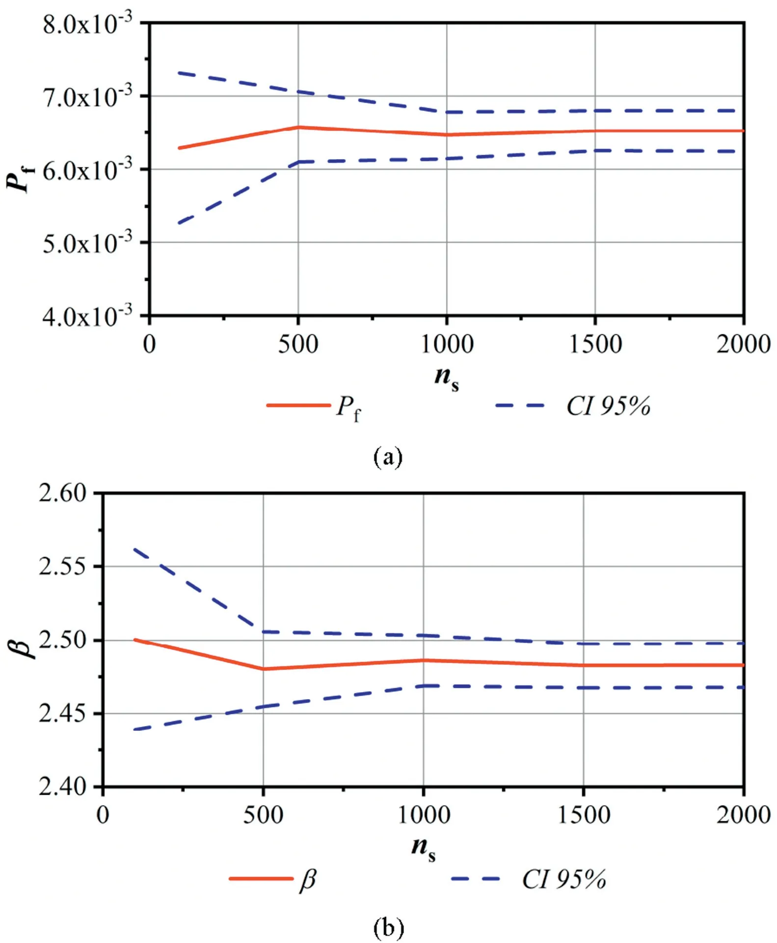
Fig.7.Convergence of ISMC simulation in terms of number of samples:(a)Failure probability(Pf)and 95% confidence interval,and(b)Reliability index β and 95% confidence interval.

The required number of samples in ISMC simulation needs to be checked in a convergence plot,where computed reliability index(β),failure probability(Pf),and sample variance are plotted against an increasing number of samples,for the mean and 95% confidence interval(CI).This convergence plot was obtained using up to 2000 samples and shows that results are stabilized after about 1000 samples,as shown in Fig.7a and b.

Results obtained for OPC 3 with FORM,SORM and ISMC simulation are compared in Table 3.The difference in reliability indices(β)between FORM,SORM and ISMC simulation is approximately 2% ,which indicates that all methods tend to converge(Table 3).An error of approximately 2% was found with FORM,and of approximately 1% with SORM,in comparison to the reference solution of ISMC simulation(Table 3).The results obtained by FORM and SORM agreed with the results obtained by ISMC simulation,showing that the long-term steady-state dam reliability problem was not excessively nonlinear.FORM was employed in the remaining reliability analyses in this study.

All design points in the above solutions were found using the HLRF algorithm.The limit state functions were not excessively nonlinear;hence,no convergence problems were observed in the analyses. In the case of nonlinear limit state functions, the improved HLRF(iHLRF)algorithm can be employed(for instance,the discussion in Ji et al.(2018,2019)).Both algorithms(HLRF and iHLRF)were available in the StRAnD software.

4.2. Sensitivity of variables

An advantage of FORM is the possibility of carrying out a sensitivity analysis through the direction cosines(α2)at the DP,revealing the contribution of each random variable to the evaluated failure probabilities.

Sensitivity results are evaluated for different OPCs,probability distributions and COV,as shown in Fig.8.Fig.8a compares the sensitivity values for the three OPCs using COVmeand LN distribution.Fig.8b compares the sensitivity values for OPC 3 and LN distribution for different values of COV. Fig. 8c compares the sensitivity values for OPC 3 and COVmefor different probability distributions.These results were computed considering random seepage properties(Ks,θs,θr,a and n)and random stability calculations(γ,c＇,φ＇and φb).Sensitivity coefficients(α2)for seepage properties(Ks,θs,θr,a and n)cannot be seen in Fig.8 because they are nearly zero(α2≈0);hence,these random variables have negligible contributions to the computed failure probabilities and can be considered deterministic.From the results in Fig.8,we also concluded that,for the dam studied herein,the uncertainty in friction angle φ＇has the greatest contribution to the failure probabilities,for all operational cases,COV values and statistical distributions considered herein.The second most important random variable was the effective cohesion c＇.The unit weight γ had small importance(α2≠0),and the angle that increased the shear strength φbincreased importance from OPC 3 to OPC 1.The unsaturated soil condition had a greater effect when the phreatic surface was in a low position.

Studies of stochastic pore pressure variability(Bergado and Anderson,1985)and stochastic hydraulic conductivity(Gui et al.,2000),as well as other studies(Srivastava et al.,2010;Yi et al.,2015),show that the seepage properties have great importance on reliability analysis.A comparison of our results with the above references reveals that the COV values in our study are smaller.

In the remaining reliability analyses,stability properties(γ,c＇,φ＇and φb)were considered as random variables,and seepage properties(Ks,θs,θr,a and n)were assumed to be deterministic,by their mean values.

4.3. Influence of the reservoir level on the reliability index

In this section,the reliability analysis considers(i)only the LN distribution and(ii)only median values of the coefficients of variation(COVme).From the results shown in Fig.9 and Table 4,we concluded that for the dam studied herein,smaller reliability indices and higher probabilities of failure were found in higher water levels.

4.4. Influence of the statistical distribution on the reliability index

In the present section,the reliability analysis considers only the median values of the coefficients of variation(COVme).It is well known that geomechanical material properties listed in Table 1 should be positive values.Nevertheless,statistical fitting to the measured data often yields the N distribution as a candidate distribution.Moreover,when N distribution is assumed,it simplifiesreliability analysis(e.g.linear limit state functions of the normal variables allow analytical,closed-form solutions).Hence,there is relevance in the discussion of using mathematically correct LN and TN strictly positive distributions,or convenient N distribution.As well reported in the literature(Guo et al.,2018;Mouyeaux et al.,2018,2019),using N distribution to represent strictly positive material properties can lead to numerical computation problems and unrealistic values.

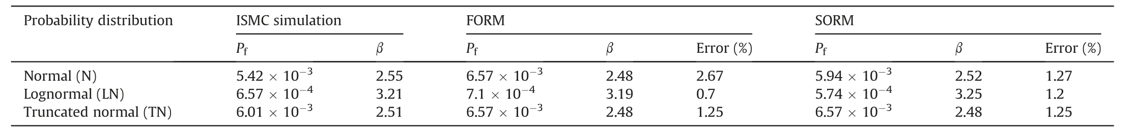
Table 3 Results of the reliability analysis for OPC 3 and COVme.

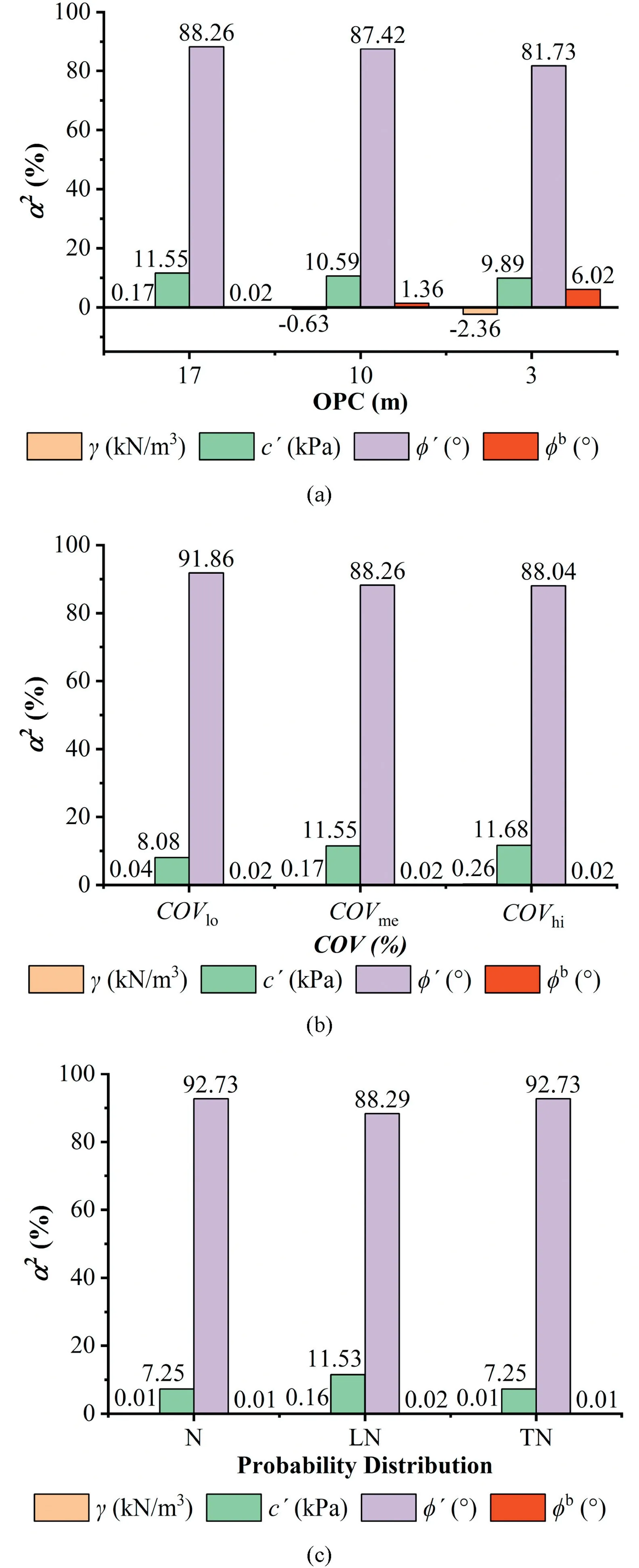
Fig.8.Sensitivity analysis results for different scenarios:(a)three OPCs with LN distribution and COVme,(b)OPC 3 with LN distribution and COVlo,COVme and COVhi,and(c)OPC 3 with N,LN and TN distributions and COVme.

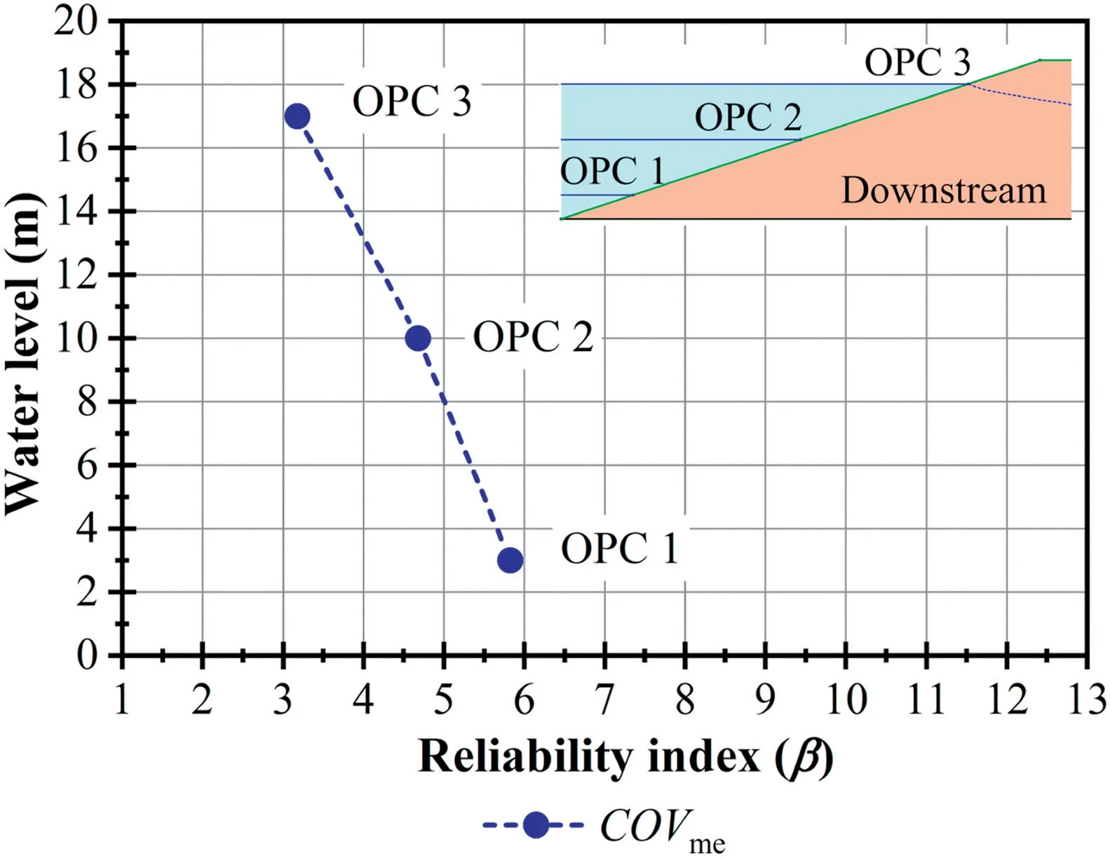
Fig.9.Reliability index with COVme and the LN distribution for three OPCs.

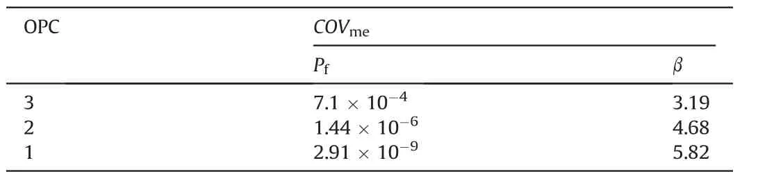
Table 4 Results of the reliability analysis with COVme and the LN distribution for three OPCs.

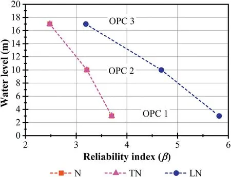
Fig.10.Reliability index with COVme for three OPCs.

Herein,we investigated the influence of the choice of probability distributions on the computation of reliability indices for dam stability.Fig.10 and Table 5 show the results obtained for the dam stability problem using N,TN or LN distribution.First,we observe that LN distribution leads to significant increases in the calculated reliability indices(up to 60% for lower reservoir level).Second,we observed no differences between reliability indices evaluated using N or TN distributions.Note that the LN distribution is asymmetric with respect to the mean,whereas the N and TN distributions are symmetric.Third,although GeoStudio does not accept negative values for geotechnical properties,we did not encounter numerical problems with our computations using N distribution.There aretwo complementary reasons for this result.One reason is that reliability indices are reasonably large,which causes the design points to be far from negative values.The second reason is the FORM and ISMC simulations employed in computation.The iterative search for the DP in FORM remained far from negative values during the whole process due to a well-behaved limit state function.Use of importance sampling also kept sampled points away from the negative region.The use of simple MCS,and/or smaller reliability indices would make it more likely for the software to yield negative values,causing numerical problems in computation.The use of TN distributions for strictly positive geotechnical properties is always advisable.In the remainder of this paper,only TN and LN distributions are employed.

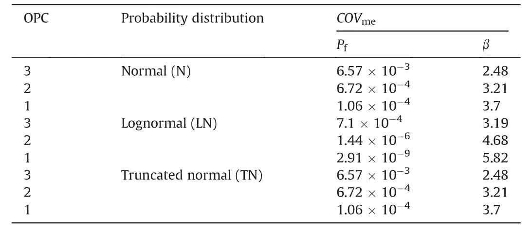
Table 5 Results of the reliability analysis with COVme for three OPCs.

Fig.11.Reliability index with LN distribution for three OPCs.

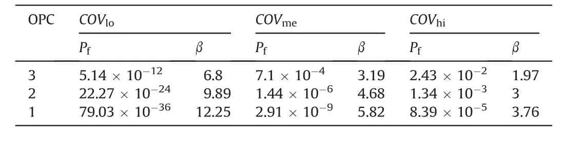
Table 6 Results of the reliability analysis with LN distribution for three OPCs.

4.5. Influence of the coefficient of variation on the reliability index

In the present section,the reliability analysis considers only the LN distribution.From the results shown in Fig.11 and Table 6,it shows that,for the studied dam,the reliability index(β)increases when the coefficient of variation(COV)decreases.The probability of failure increases when higher values of COV are used in reliability analysis.The results for different COV values indicate how sensitive the analysis is to the assumed values of soil uncertainty-related parameters(Salgado and Kim,2014).The dependence of β on the COV values depends on the problem.For nonlinear problems,reliability indices will vary in a nonlinear way with the reciprocal of COV,as shown in our results.Using extreme values produces 245% of the change in β between COVhiand COVlo.

The determination of COV in a reliability analysis of an earth dam is one of the most important steps.The use of extreme values from the literature due to the lack of laboratory or field studies has an important influence on the reliability analysis.The experiences of engineers and the number of laboratory and field tests help in choosing the correct COV for geotechnical materials and make decisions.

4.6. Influence of correlation on reliability index

In the present section,the reliability analysis considers(i)only OPC 3;(ii)only median values of the coefficients of variation COVme;and(iii)the correlations between the cohesion and friction angle(ρc＇-φ＇),cohesion and unit weight(ρc＇-γ),unit weight and friction angle(ργ-φ＇)and the correlations among all of them.

From the results shown in Table 7,it is inferred that,for the studied dam,the reliability index(β)increases considerably when the correlation ρc＇-φ＇is considered,in the case of LN and TN distributions.The results in Tables 8 and 9 show that correlations ρc＇-γ and ργ-φ＇have much smaller impacts on the reliability indices.

Three different problem configurations are considered in the reliability analysis.The results are shown in Table 10,Figs.12 and 13.Correlation case ρaconsidersand ργ-φ＇=0.4.Correlation case ρbconsidersand ργ-φ＇=0.4.Correlation case ρcconsidersand ργ-φ＇=0.4.

From the results shown in Table 10,Figs.12 and 13,it illustrates that for the studied dam,the reliability index(β)increases considerably in the LN and TN distributions when different combinations of correlations(ρa,ρband ρc)are used.The results show that the correlations between obtained geotechnical properties significantly impact structural reliability,suggesting the importance of further investigation of such correlations in the field.

From the results shown in Table 10,Figs.12 and 13,it can be concluded that for the studied dam,the use of all correlations(ρc＇-φ＇,ρc＇-γ and ργ-φ＇)in the same analysis,or consideration of ρc＇-φ＇only,leads to similar reliability index results,but the computational cost increases.

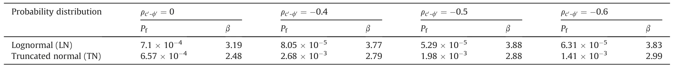
Table 7 Results of the reliability analysis with different correlations of the cohesion and the friction angle(ρc＇-φ＇)for COVme and OPC 3.

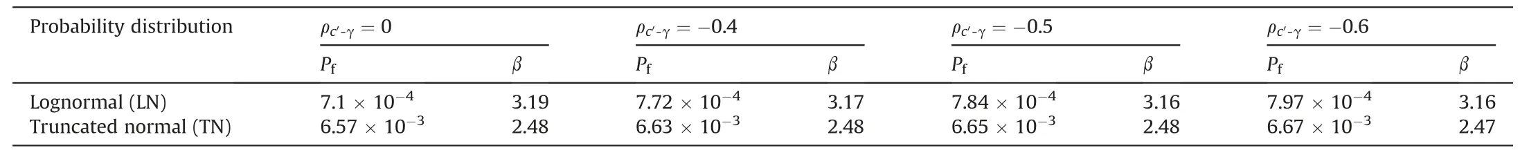
Table 8 Results of the reliability analysis with different correlations of the cohesion and the unit weight(ρc＇-γ)for COVme and OPC 3.

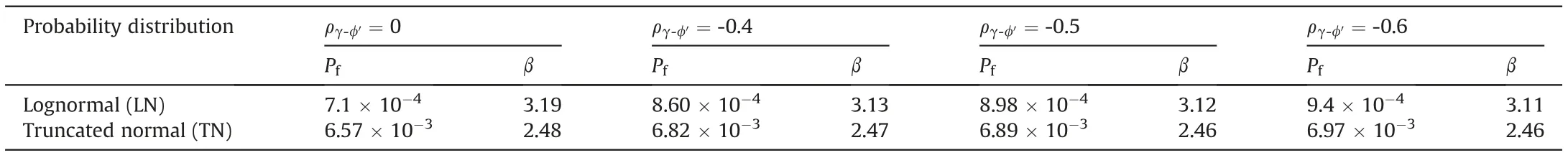
Table 9 Results of the reliability analysis with different correlations of the unit weight and the friction angle(ργ-φ＇)for COVme and OPC 3.

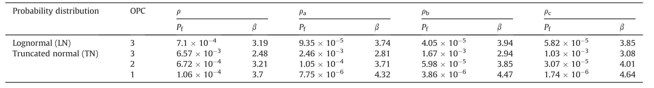
Table 10 Results of the reliability index with COVme and different correlations and OPCs.

For correlated random variables,the transformation to standard Gaussian space involves two additional computations:evaluation of equivalent correlation coefficients and Cholesky decomposition of the equivalent correlation matrix.This explains the impact in terms of computational cost of using correlations between variables;hence,it is inefficient to include correlations with negligible impacts on reliability.Only perfect correlations can reduce costs:in this case,the dependent random variable can be written as a function of the other,and problem dimensionality is reduced.However,this is not the case in our examples.

4.7. Determination of the critical surface

In this section,the reliability analysis is performed for(i)the LN distribution only,and(ii)the median values of the coefficients of variation (COVme). A comparison of the corresponding critical deterministic and probabilistic slip surfaces,for the three OPCs,is presented in Fig.14a,b and c,respectively.

Reliability analysis using FORM involves a search for the DP.When the random variables assume the values corresponding to the DP,the slip surface with the highest probability of occurrence is obtained,which is referred to as the probabilistic slip surface.

Hassan and Wolff (1999) and Bhattacharya et al. (2003)employed the mean value second-moment theory(MVFOSM)to find the probabilistic critical slip surface,assuming all random variables to be Gaussian distribution. In contrast, the direct coupling developed herein allows us to consider non-Gaussian distributions,which results in more accurate critical slip surfaces,either using FORM or MCS.

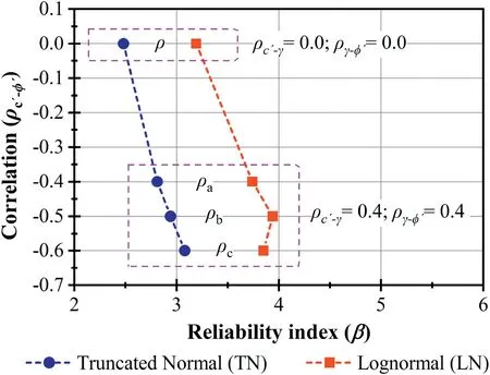
Fig.12.Reliability index with COVme for OPC 3 and different correlations of ρc＇-γ,ρc＇-φ＇and

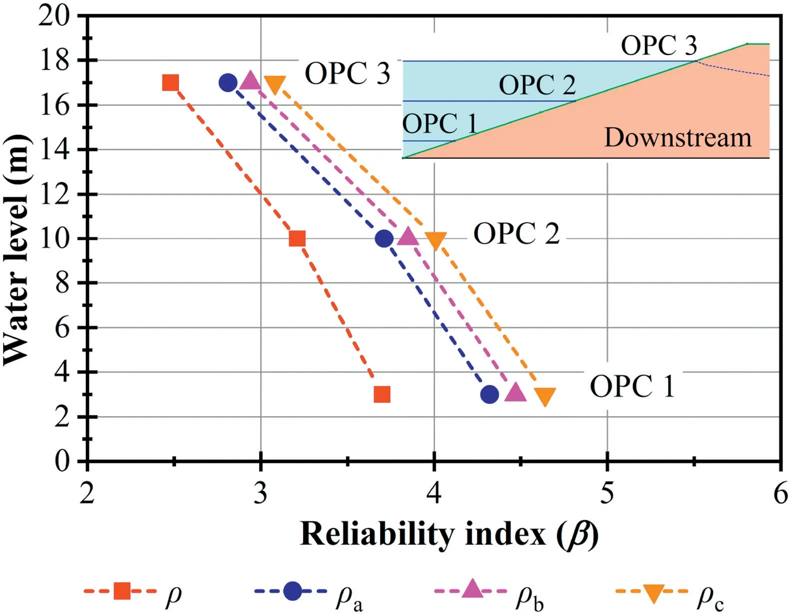
Fig.13.Reliability index with COVme and the TN distribution for different correlations and OPCs.

Fig.14.Comparison of dam slip surfaces obtained from deterministic and probabilistic approaches,with the LN distribution and COVme,for three OPCs:(a)OPC 3,(b)OPC 2,and(c)OPC 1.

When the seepage and stability analyses are performed for the mean values of the random variables,the slip surface leading to the minimum FS is called the critical slip surface.As evident in Fig.14,these surfaces are not the same. For the homogeneous slope considered herein,the difference is not too large,but in general,they will be different.Performing the reliability analysis using the deterministic slip surface leads to incorrect results. Although Fig.14a,b and c gives the impression that the critical slip surfaces are the same,they are slightly different for each OPC.

5. Conclusions

This paper addressed accurate and efficient solutions of geotechnical reliability problems by means of DC of deterministic geotechnical software with a probabilistic solver.DC allows solving the reliability problem by means of accurate and efficient methods such as FORM and ISMC simulation.The coupling feature was illustrated by coupling the deterministic GeoStudio 2018 software with the StRAnD reliability analysis software.The coupling was also illustrated in the equilibrium analysis of an earth dam.

Equilibrium analysis of the earth dam was done for three different OPCs.Long-term steady-state seepage and stability analyses were performed.Dam reliability was found to change significantly with water level above the bedrock.The results obtained by FORM and SORM agreed with those obtained by ISMC simulation,showing that the earth dam stability problem is almost linear in random variable space.This observation included linearity of the limit state functions and of the transformation of LN variables to standard normal space.

Sensitivity analysis revealed that the four“stability analysis”variables(c＇,φ＇,γ and φb)dominated failure probabilities,whereas the five“seepage analysis”random variables(Ks,θs,θr,a and n)had little influence.In all studied cases,the friction angle(φ＇)and cohesion(c＇)were found as the most influential parameters in the reliability analysis.

The influence of the reservoir level clearly showed that higher reliability indices were found for lower levels of the reservoir,and lower reliability indices for higher levels of the reservoir.The use of different probabilistic distributions for the geotechnical materials showed higher values of reliability indices using LN distribution, and similar values for N and TN distributions. The truncation of“negative”material properties,by using TN instead of N distributions,showed little influence on the“high reliability”dam studied herein.This may not be the case for dams with lower reliability.

The coefficients of variation(COV values)of random properties were shown to produce large impacts on dam reliability.Smaller COV values led to larger reliability indices.The assumption of COV values from the literature may be accepted as an initial approach,but these assumptions have to be confirmed by field tests.

Correlation between material properties was also considered.Correlation between cohesion and friction angle(ρc＇-φ＇)showed the largest impact associated with increasing reliability indices.On the other hand,correlations between cohesion and unit weight(ρc＇-γ),and between unit weight and friction angle(ργ-φ＇)led to negligible variations in β.

Finally,it was shown that the most probable slip surface,found in the reliability analysis,was not the same as the critical slip surface found in a mean value analysis for the minimum FS.

Declaration of Competing Interest

The authors wish to confirm that there are no known conflicts of interests associated with this publication and there has been no significant financial support for this work that could have influenced its outcome.

Acknowledgments

The authors thank the financial support by the Coordination for the Improvement of Higher Education Personnel (CAPES) for research funding(Grant No.88882.145758/2017-01)and the Brazilian National Council of Scientific and Technological Development(CNPq).