Comparisons of Three-Dimensional Variational Data Assimilation and Model Output Statistics in Improving Atmospheric Chemistry Forecasts

Chaoqun MA,Tijian WANG?,Zengliang ZANG,and Zhijin LI

1School of Atmospheric Sciences,Nanjing University,Nanjing 210023,China

2CMA-NJU Joint Laboratory for Climate Prediction Studies,Nanjing 210023,China

3Jiangsu Collaborative Innovation Center for Climate Change,Nanjing 210023,China

4Institute of Meteorology and Oceanography,PLA University of Science and Technology,Nanjing 210000,China

5Joint Institute for Regional Earth System Science and Engineering,University of California,Los Angeles 90001,California,USA

1.Introduction

In recent years an unexpected outbreak of severe air pollution events has engulfed China during the autumn and winter months of the year.These air pollution episodes have aroused deep concern and panic amongst the public and have subsequently become a top priority to address for the government.For example,the State Council released the Air Pollution Prevention and Control Action Plan in September 2013,aimed at reducing particulate pollution.In addition,targets to control sulfur dioxide and nitrogen oxides were listed in the 11th and 12th Five-Year Plan drawn up by the National Development and Reform Commission.However,to control atmospheric pollution efficiently,it is necessary to achieve more accurate forecasting of atmospheric chemical constituents.

Since the beginning of the 21st century,air quality forecast systems,such as the Weather Research and Forecasting-Chemistry(WRF-Chem)model,have been gradually put into operation in key cities across China by many organizations and institutions.However,without any additional measures,these numerical forecast systems are not accurate enough to be applied in operational air quality forecasts due to the uncertainties within their parameterization schemes and input data(van Loon et al.,2007;Zhang et al.,2016).Accordingly,scientists have developed multiple pre-or post-processing techniques for model improvement in the operational prediction of meteorological and chemical fields.For example,data assimilation(DA)—a measure applied before the model run—is an effective approach in improving the model forecast skill of air pollution via reducing the uncertainty of chemical initial conditions(CICs)or other parameters.For instance,Barbu et al.(2009)achieved a better forecast by assimilating measurements of sulfur dioxide(SO2)and sulfate to adjust the emission and conversion rates of SO2in the model;and the research of Liu et al.(2011)and Yin et al.(2016)showed improved aerosol analysis and forecasting by assimilating the MODIS total aerosol optical depth retrieval products.Different models and observational data have been tested and their results show similar conclusions(Wang et al.,2014;Zhang et al.,2015;Mizzi et al.,2016;Tang et al.,2016)—readers who are interested should refer to Bocquet et al.(2015)for more details.Alternatively,the forecast error can also be corrected effectively by another approach,called model output statistics(MOS)(Glahn and Lowry,1972).MOS works through statistically relating the historical model output with corresponding observations,and then applying the relationship to the model forecast.This approach has been widely used in the post-processing of operational numerical weather prediction,and in doing so most forecast biases can be corrected(Wilson and Vall′ee,2003),especially for temperature(Taylor and Leslie,2005;Libonati et al.,2008)and humidity(Anadranistakis et al.,2004).

Although it has been proven that both DA and MOS are effective in improving the forecast performance,little attention has been paid to comparing or combining the two methods,especially with respect to atmospheric chemistry modeling.There are two obstacles that make it difficult to compare the two methods fairly using the same observational dataset.First,most early(and even recent)research concerning 3DVar in atmospheric chemistry models has focused on assimilating observations from satellite-derived products to generate analyses that are skillful in improving the forecasts of variables like carbon monoxide(Barret et al.,2008),carbon dioxide,ozone(O3),nitrogen dioxide(NO2)(Inness et al.,2015;Wargan et al.,2015),methane(Alexe et al.,2015),and aerosols(Benedetti et al.,2009;Yumimoto et al.,2016).However,MOS works only with in-situ observations from surface stations.Second,unlike numerical weather prediction,MOS still remains in its infancy in terms of the operational numerical forecasting of atmospheric chemistry variables.Such works,if any,are usually based on regression approaches(Denby et al.,2008;Honore et al.,2008;Struzewska et al.,2016),which are effective in improving the air quality forecast for all analyzed species.However,methods based on these approaches are usually too dependent on local pollution conditions,which makes them inconvenient to be applied as widely as DA approaches.

This study compares the potential of the two approaches in improving the atmospheric chemistry forecasts of the WRF-Chem modeling system in an operational context.To overcome the problems mentioned above,we firstly adapted a 3DVar DA system based on Li et al.(2013)(L13 henceforth)and Jiang et al.(2013)to the assimilation of observational data from surface stations.Then,we modified a MOS scheme from Galanis and Ana dranistakis(2002)(hereafter G02)for use in adjusting the meteorological forecast,to enable it to correct the chemistry output from the atmospheric model.Following this introduction,the model,setup and experimental design are described in section 2.Section 3 evaluates the model improvement with the two methods.A summary and conclusion are given in section 4.

2.Method and data

2.1.Model setup

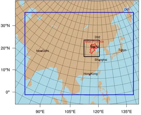
Fig.1.The nested domains of the WRF-Chem model:D01(blue frame)is the outer domain,which covers most of East Asia;D02(black frame)is the inner domain,in which Hebei Province(red boundary)is located.

The WRF-Chem model is an online 3D,Eulerian chemical transport model that considers the complex physical and chemical processes in the troposphere(Grell et al.,2005).It has been applied in various research settings,especially those concerning feedbacks of air pollution to meteorological and chemical DA(Saide et al.,2012,2015;Makar et al.,2015;Mizzi et al.,2016).In this study,version 3.7.1 of WRF-Chem was used to simulate the air quality in Hebei Province,China.Two nested domains were set,as shown in Fig.1.The outer domain covered East Asia with a hori-zontal resolution of 75 km×75 km and 106(lon)×81(lat)grids,while the inner domain covered Hebei Province with a horizontal resolution of 15 km×15 km and 76(lon)×81(lat)grids.The vertical resolution of the model was 24 vertical levels(about 6 levels below 1 km and 20 levels below 10 km),with 100 hPa as the model top.The 0.5°×0.5°data from the NCEP’s Global Forecast System were used to provide the meteorological initial conditions and lateral boundary meteorological conditions every 12 hours.Atmospheric gaseous chemistry and aerosols were simulated using the Second Generation Regional Acid Deposition Model(RADM2)with the Modal Aerosol Dynamics Model for Europe(MADE)and the Secondary Organic Aerosol Model(SORGAM)(Stock well et al.,1990;Ackermann et al.,1998;Schell et al.,2001)scheme.The anthropogenic emissions inventory was the Multi-resolution Emissions Inventory for China in 2012(http://www.meicmodel.org).The con figuration of WRF-Chem is detailed in Table 1.

2.2.MOS method

What MOS does is to find statistic relationships from training samples that can then be applied in model forecast outputs.By doing so,the expectation is that model errors will be corrected and a forecast generated that will better fit the observation.In this study,a one-dimensional Kalman filter was chosen as the algorithm to realize the MOS process.The algorithm was formulated in a way that generally resembled G02;the only modi fications were as follows:

Firstly,in this work,the measurementy(t),as well as the real valuex(t),could both be the difference and ratio between the forecast and observation,whereas in Eqs.(1)and(2)of G02 they only denoted the difference.Furthermore,hourly concentrations of five species from the three-day model output were split into 3×5×24 independent daily concentration series.Lastly,given Kalman filtering can only predict one time-step ahead(one day ahead,in this context),the correction could only work during forecast hours 0–24(24-h forecast hereafter),while leaving forecast hours 24–48 and 48–72(48-h and 72-h forecast hereafter)uncorrected.Therefore,to extend the algorithm further,the corrected results from the 24-h(48-h)forecast was used as a proxy or substitute observation at the corresponding time to correct the 48-h(72-h)model output.Appendix A describes the steps in more detail.

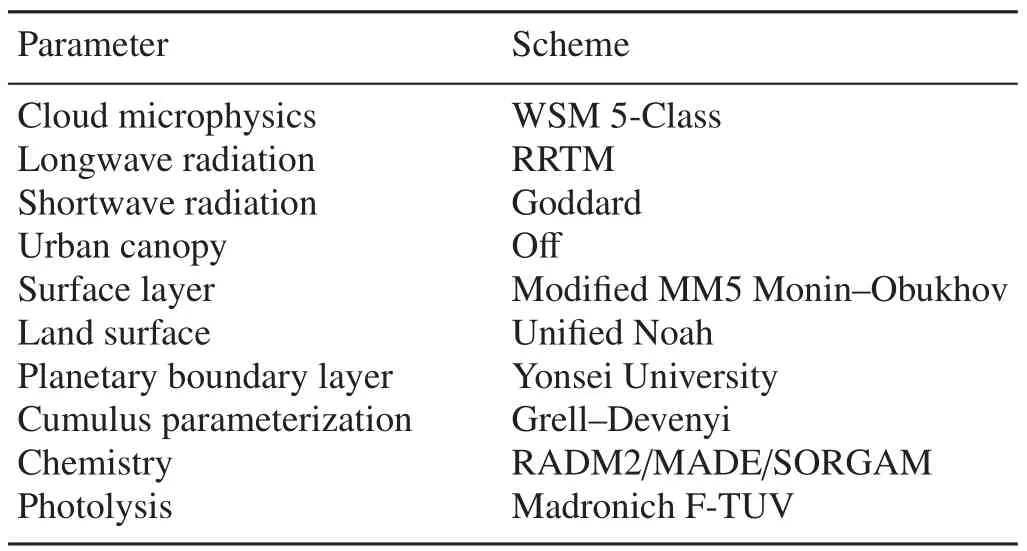
Table 1.Con figuration of the physical and chemical schemes of WRF-Chem.

2.3.DA con figuration

In this study,3DVar DA was implemented to optimize the CICs for the inner model domain.The DA system and formulation used were based on L13 with the following modi fications:

In addition to the fine particulate matter(PM2.5)assimilated in L13,particulate matter with diameters between 2.5μm and 10 μm(PM2.5–PM10)was also assimilated and the analysis increment was added to the corresponding model variables following L13.Gaseous species,including SO2,NO2and O3,were also assimilated to decrease the uncertainty of their concentrations in the model CICs.

Following L13,the National Meteorological Center(NMC)method(Parrish and Derber,1992)was adopted to estimate the background root-mean-square error(RMSE)and the three Kronecker product members of the background error correlation matrix.The NMC method utilized the difference between the 12-and 24-h WRF-Chem forecasts valid at the same time of 1200 UTC for a whole month.No cross correlation between different species was assigned for background error.The domain-average RMSEs for five species are shown in Fig.2.The vertical distributions of RMSE for all species display a relatively rapid decrease with height—except for O3,which peaks at around 4 km above the ground.The vertical correlation matrices are displayed in Fig.3.The correlation between different height levels experiences a jump at the top of the boundary layer,which seems to be a common feature for all species.In addition,the band of high correlation along the diagonal seems wider in the middle troposphere than the upper or lower troposphere.

Considering that all the stations were built and maintained under the same standards,no difference in the measurement and representativeness error between different stations was assumed.In addition,cross correlation between different species and stations was set to zero because of the lack of information.Therefore,observation error consisted merely of five values—one for each species.The measurement error was assigned as 1.0μg m?3,1.0μg m?3,1.0 ppb,1.0 ppb and 1.0 ppb for PM2.5,PM2.5–PM10,SO2,NO2and O3,respectively.Representativeness error was estimated following Elbern et al.(2007)and Schwartz et al.(2012)using the formula

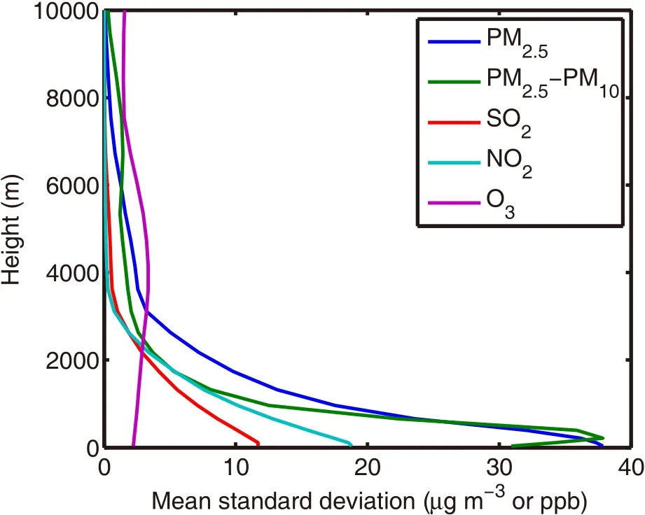
Fig.2.Vertical distribution of the root-mean-square ofthebackground errors,in mass concentration for particulate matter and ppb for gaseous species.

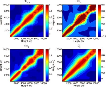
Fig.3.Vertical correlations of the background errors for PM2.5,SO2,NO2,and O3.The plot for PM2.5–PM10is very similar to that of PM2.5and so is not shown here.Both the x-and y-axis are limited within 10 km,though the real model top is higher.

where ε0and εrare the measurement error and representativeness error,γ is an adjustable parameter that accounts for the lifetime of the species(0.5 for PM2.5,PM2.5–PM10and O3;1 for SO2and 2 for NO2),Δxis the grid spacing(here,15 km),andLis the radius of in fluence determined according to the location of stations(here,4.0 km for suburban stations—assumed for all sites).If the total observation error is defined as the sum of measurement error and representativeness error,the standard deviation of observation error is 2.0μg m?3,2.0μg m?3,3.0 ppb,4.9 ppb and 2.0 ppb for PM2.5,PM2.5–PM10,SO2,NO2and O3,respectively.Though the observation error was determined fairly arbitrarily and empirically here,the uncertainty relating to it should not have a signi ficant in fluence on the conclusion.That is because the results are usually not very sensitive to the speci fication of error(Geer et al.,2006),and similar analysis fields were obtained from our experiments when the observation error was increased or reduced by a factor of two or three.

2.4.Experimental design

To compare the relative importance of MOS and DA,four parallel experiments were designed:Sim base,SimDA,Sim-MOS and Sim-DM.Simbase worked as the base simulation without applying DA or MOS;Sim-DA was an experiment with only DA employed to optimize the model CICs;Sim-MOS was the same as Sim-base but with the model output corrected by one-dimensional Kalman filtering;and Sim-DM used both the DA and MOS methods.

To simulate the operational forecast scenes,as Fig.4 shows,all experiments initiated a new WRF-Chem forecast at 1200 UTC,every day,between 30 November 2014 and 31 December 2014.Each forecast was integrated for 84 h to generate 72-h forecasts for each day,with the earliest 12 h discarded as spin-up time.The CICs for each initiation came from the 24-h forecasts of the previous cycle,which would be the background fields to be assimilated with valid observations for experiments with DA before initializing WRFChem.The first CICs at 1200 UTC 30 November 2014 came from a two-days’spin-up of the climatological background chemistry pro file.For all experiments,the chemical boundary conditions came from the default climatological chemistry pro file for the outer domain and the interpolation of the outer domain for the inner domain.

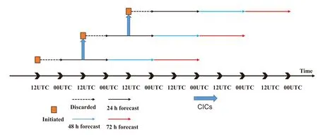
Fig.4.Time settings of the model in the four experiments.In each forecast cycle,the model was integrated 84 h in advance,with the first 12 h discarded(black dashed arrow)and the remaining 72 h divided into three parts:24-h forecast(black solid arrow),48-h forecast(blue solid arrow)and 72-h forecast(red solid arrow).The blue thick arrows mean using CICs directly for experiments without DA,while for others as the background fields of the 3DVar DA.

2.5.Observational data

Hourly concentrations of SO2,NO2,PM10,O3and PM2.5at surface level from 207 sites were provided by the Ministry of Environmental Protection of China.Data covered the whole month of December 2014 and had been subjected to routine quality control.As shown in Fig.5,only 155 stations were selected(randomly)from the 207 stations to be assimilated,and the data of the remaining 52 were used to verify the assimilation process.Because all stations were located at surface level,the adjustment of the CICs from the 3DVar DA was limited within several layers near the surface according to the vertical background error covariance.Furthermore,it should be noted that only those 155 sites that provided their data for the 3DVar DA participated in the MOS process.

3.Results

3.1.Model evaluation

Table 2 presents the mean bias(MB),relative bias(RB),RMSE and correlation coefficient(Corr)for the 24-h,48-h and 72-h forecast of Sim base.In general,the base model simulation provides a fairly good result—especially for NO2,whose bias is small and correlation high.In terms of particulate matter and SO2,the model tends to systematically underestimate the concentration of SO2as well as that of PM2.5and PM10.Even so,the model reproduces the temporal variations of particulate matter well,with Corr values higher than 0.47 for PM10and 0.54 for PM2.5.For O3,the model encounters a problem—the surface O3simulated concentrations(5–45μg m?3from observation)are seriously overestimated by the model(20–80 μg m?3from simulation),which leads to positive bias(～ 40 μg m?3)and lower Corr(0.44)than for other species.Fortunately,when viewing the RMSE of O3from the aspect of MB,it is apparent that MB contributes the largest portion of RMSE,and therefore the model is still able to reproduce the variation of O3.The biases mentioned above can usually be attributed to the uncertainties from the emissions inventory,meteorological forecasting(Tang et al.,2011)and model schemes(Yerramilli et al.,2010).Although the 24-h forecast performs the best for all species,the 48-h and 72-h forecasts are also good enough to yield fairly reliable results,which is critical to the success of MOS in the whole 72 hours’forecast.In short,the model shows forecast skill that is sufficient to be competent for the success of the DA and MOS process.

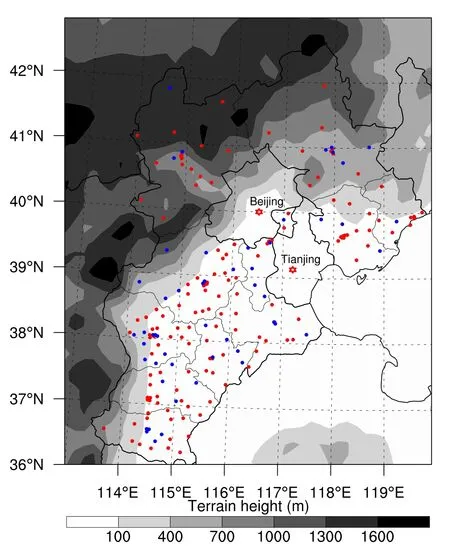
Fig.5.The terrain height of the Hebei Province,with monitoring sites plotted as filled dots.Red dots are sites that participated in the 3DVar and MOS process,while the blue ones are those used only in the validation of the DA effect.

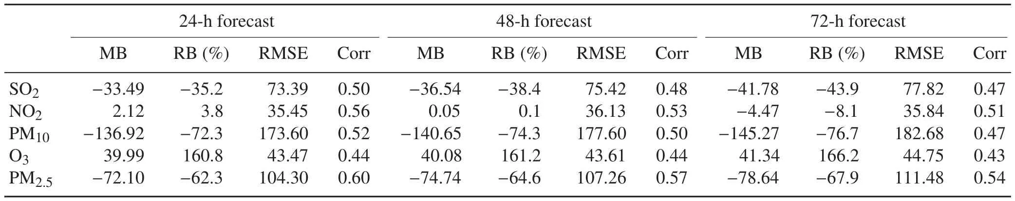
Table 2.Site-averaged mean bias(MB),relative bias(RB),root mean square error(RMSE)and correlation coefficient(Corr)for the 24-h,48-h and 72-h forecasts of five species in Sim base.Statistics were calculated according to the hourly concentration from each of the 207 sites before being averaged.Units areμg m?3for MB and RMSE.

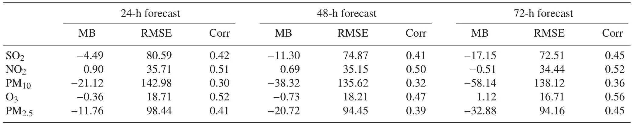
Table 3.Site-averaged MB,RMSE and Corr for the 24-h,48-h and 72-h forecasts of five species in Sim MOS.Statistics were calculated according to the hourly concentration from each of the 207 sites before being averaged.Units areμg m?3for MB and RMSE.

3.2.Validation of MOS

Figure 6 depicts the site-averaged hourly concentration simulated by Sim MOS,plotted against ground observations.Note that,although the hourly concentrations were averaged over 155 stations,the MB and RMSE values in Table 3 were generated by first calculating the individual errors of the 155 stations,before averaging.

From Fig.6 it can be concluded that the forecast from Sim MOS fits the observation fairly closely—especially for SO2,NO2and O3.However,when it comes to PM2.5and PM10,the points locate within a wider space,and those extremely high observations are hard for MOS to forecast.Even so,when comparing Table 3 with Table 2,PM2.5and PM10,together with the other three species,demonstrate that a clear correction can be obtained for all forecast times.Excluding the 48-h forecast of NO2,MOS can reduce the MB to a large extent,meaning this method can remove the majority of the model systematic bias.Because of the reduction in MB,the RMSE also decreases for all cases except the 24-h forecast of SO2.In addition,the effect on reducing the error is unlikely to become poorer as the forecast time advances.For the 72-h and 48-h forecasts,the effect MOS has on the former may rival or even exceed that on the latter,e.g.,the RMSE reduction of PM2.5is even larger for the 72-h than 48-h forecast.For the 48-h and 24-h forecasts,the same effect can be found.Among all five species,O3seems to bene fit the most from the MOS process.This is because O3usually follows a very regular daily variation,which makes the hourly-split but dailylinked concentration series almost perfect for the assumptions of one-dimensional Kalman filtering.

Admittedly,MOS degrades the forecast in a few cases(e.g.,the 48-h forecast of NO2and 24-h forecast of SO2,as mentioned above).Such increases in error,however,will usually not be of concern to users,and may well be accepted,as they are extremely small and only appear at times when the model outputs to be corrected are already fairly close to the observation.Nonetheless,when viewed from the correlation perspective,such degradation becomes moreobvious.Except for NO2and O3,the correlations all experience a reduction by 0.1–0.2.Thus,the MOS approach tends to reduce the bias and error at the expense of correlation.

3.3.Validation of DA

Figures 7 and 8 show the change in RMSE and Corr over the integration time from?12 h(right after the DA)to 10 h(already integrated for 22 h),respectively,for experiments Sim base and SimDA.To keep the veri fication independent from the observations assimilated,the RMSE and Corr were only averaged over the 52 stations that did not provide their observational data in the 3DVar DA process.

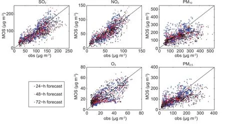
Fig.6.Hourly concentrations simulated by Sim MOS,plotted against ground station observations(obs)averaged over 155 stations.

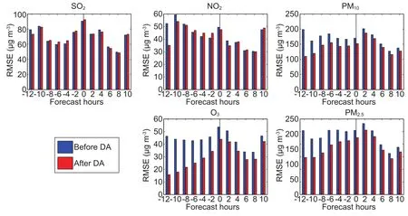
Fig.7.RMSE change over the integration time from the?12 h forecast(right after the DA)to the 10 h forecast(already integrated for 22 h)for the five species.All RMSE values were averaged over the 52 stations that did not provide observations in the DA.

From the?12 h forecast of Fig.7 and Fig.8,DA leads to better initial conditions for the simulation—especially for NO2,PM10,PM2.5and O3,whose RMSEs decrease substantially at almost all sites.For example,PM10and PM2.5shown an RMSE reduction of about 50–100 μg m?3,which is about half the RMSE of Simbase.Such results are as good as those obtained by L13 and Jiang et al.(2013),who also worked on assimilating ground observations using 3DVar.For SO2,the reduction in RMSE is less apparent(although the change in RMSE is still negative when 52 sites are averaged),but the correlation after DA is still obviously larger than before.The marginal RMSE reduction for SO2may be acceptable considering the increase in correlation is rather obvious and the data representativeness of some stations is dubious(Zhang et al.,2016).

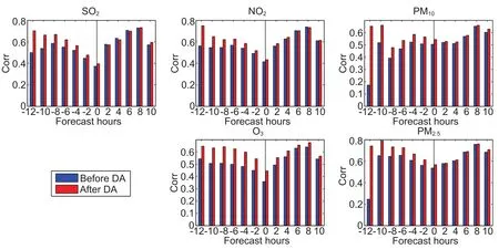
Fig.8.Similar to Fig.7 but for Corr.

However,as expected,the effect of DA slowly diminishes as the integration continues,which has also been observed in other works(Jiang et al.,2013;Li et al.,2013).After the model has been integrated for more than 14 h,the RMSE after DA minus that before DA(RMSE change henceforth)is still negative,but their absolute values are apparently smaller when compared to the earlier ones.The effect of DA remains for longer in the case of O3,PM10and PM2.5(RMSE change remains negative for the 14 h),benefiting mainly from their relatively long lifetimes.For example,PM2.5and PM10still maintain an RMSE reduction of about 10–20 μg m?3,which is even better than the results reported by L13 and Jiang et al.(2013).However,for NO2,whose lifetime is short,the two experiments show almost no difference in RMSE after four hours’integration.Because the initial improvement from DA is relatively small,the forecast of SO2soon loses its improvement from DA and shows little RMSE change almost immediately after the run of the model.For SO2and NO2,the RMSE change is positive in some cases,but the increase in RMSE is usually very small compared with the original RMSE,and therefore unlikely to be a problem.Conclusions from the viewpoint of correlation are similar to those from the RMSE,except the effect of DA seems more obvious and long-lasting.

Overall,for most cases,DA successfully produces better CICs for the model and may help to improve the forecast skill in the following half to one day.

3.4.Effect of MOS and DA

From Fig.9,which plots the RMSE of the four experiments and five species at different forecast hours from ?12 h to 72 h,we can see that the forecast error varies with forecast hours.Considering the RMSE was calculated from the statistics of one month,Fig.9 is a good representation of the general features of the four experiments.

By comparing the experiments using MOS(solid lines)with those without MOS(dotted lines),it is clear that all species show a large reduction in the 72 hours forecast span,and that this reduction is much larger than can be provided by DA(solid lines are below the dotted lines by a larger distance than the blue lines are below the red).For example,when compared to Sim base,the average SO2RMSE decreases by 4.34 μg m?3for Sim MOS(average taken over all stations throughout the whole 72-h forecast),while the decrease is only 0.48μg m?3for Sim DA.Worse still,when the forecast runs to its second or third day,the effect of DA inevitably diminishes(as evidenced by the overlapping red and blue dotted lines after 24 h),while MOS can still work during this period(solid lines do not overlap the dotted lines,even after 24 h).

The blue dotted lines represent the simulation RMSE corrected only with MOS,while the red dotted lines are the results processed by both MOS and DA.Overlapping of the two lines can be seen at almost all times from all species,meaning the DA of the initial conditions provides little help to the effect of MOS,although does provide better initial conditions for the model to generate a better forecast.However,sometimes the two lines do not overlap,and show some differences,which is common for all species but most obvious for NO2and most unobvious for PM10and PM2.5.When DA can still improve the forecast,or the red dotted line is below the blue dotted line,the red solid line could be either above(1-h forecast for SO2)or below(10-h forecast for O3)the blue line,which means a better forecast from DA may either improve or degrade the MOS effect.Because in this work MOS corrects one day’s forecast using the correction results and forecast from previous days,it is not a surprise that Sim DM and SimMOS show discrepancies when SimDA and Simbase coincide after 24 h.However,as mentioned,such a discrepancy could be either an improvement or degradation.

3.5.Discussion

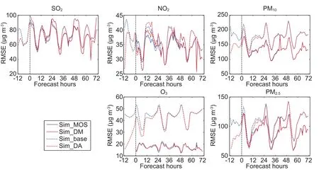
Fig.9.RMSE of the four experiments and five species at different forecast hours from ?12 h to 72 h.

This section provides additional discussion around two facts.First,that MOS may improve forecasts far more than the 3DVar DA of CICs.This is reasonable because MOS can remain effective throughout the whole forecast period,whereas the effect of 3DVar via optimized initial conditions usually diminishes after 24 h of model integration.The loss of bene fit from 3DVar DA is unavoidable because atmospheric chemistry is less sensitive to CICs than other driving factors like meteorological conditions and emissions(Henze et al.,2009;Semane et al.,2009;Tang et al.,2011).Worse still,the forecast during the earliest 12 h,which bene fits the most from 3DVar DA,usually makes no sense in a real operational forecasting environment and is excluded from evaluation as spin-up.In fact,when compared with Sim base,Sim DA can account for 43.85%of the O3RMSE reduction in the first 12 h after initialization(forecast hour?12 to?1),closely rivalling the contribution of Sim MOS(55.94%)in its first 12 h(forecast hour 0 to 11).However,when discussed within the same forecast period,e.g.,12 h to 24 h,Sim DA can produce only 3.93%of the O3RMSE reduction,which is far less than Sim MOS(61.26%),despite the following hours during which DA has no effect at all.

The second fact to be explained is that Sim DM does not al way so ut per form Sim MOS.This result is somehow against the experience that,when corrected with the same MOS algorithm,better input should lead to better or at least not worse output.However,for example,assume the difference between the forecast and observation remains constant before 3DVar is applied.(This condition may never happen in reality,but this does not matter for the purposes of demonstration).Then,no matter how large the constant is,the MOS method might work perfectly to eliminate it.However,after DA is applied,it is possible that the difference may reduce though no longer remain constant.In this case,although the forecast becomes better before MOS,it is now more difficult for MOS to eliminate the error.So,it should be noted that the error’s temporal consistency,rather than its magnitude,determines the effects of MOS on the model outputs.When reducing the magnitude of the error of model outputs,the 3DVar DA process may at the same time violate or increase its consistency to degrade or improve the effects of MOS from case to case.Therefore,such a phenomenon is uncorrelated with the inherent or necessary nature of the model,DA and MOS processes,and will be changed randomly whenever the three change their setup.The assumption is supported by the evidence that the results are very different when the whole experiment is replicated but with the spatial resolution of the original anthropogenic emissions changed from 0.1°×0.1°to 0.25°×0.25°[see Fig.10(PM2.5and PM10not plotted given the problem for them was not obvious in Fig.9)].For example,in Fig.9,SO2is predicted better by Sim DA than Sim base at the second forecast hour,but Sim DM is beaten by Sim MOS.However,in Fig.10,the same comparison leads to an inverse result,which shows Sim DM performs better than Sim MOS.Given the fact that the experiments cover a period of only 1 month,it is possible that the forecast ability of Sim MOS is slightly worse than, or almost the same as,Sim DM,if the experiment is carried out over a longer time.However,results from short-term experiments,which contain random error just like everyday forecast,still demonstrate that using MOS and DA together does not guarantee a better output than MOS only,which should be carefully considered by researchers and forecasters working in this field.

4.Conclusion

A comparison between the effect of MOS and DA in improving the forecast skill of an atmospheric chemistry model was performed in a near real operational context.The evaluation based on observations showed that both 3DVar DA and MOS based on one-dimensional Kalman filtering are effective measures to reduce the errors in the model forecast.

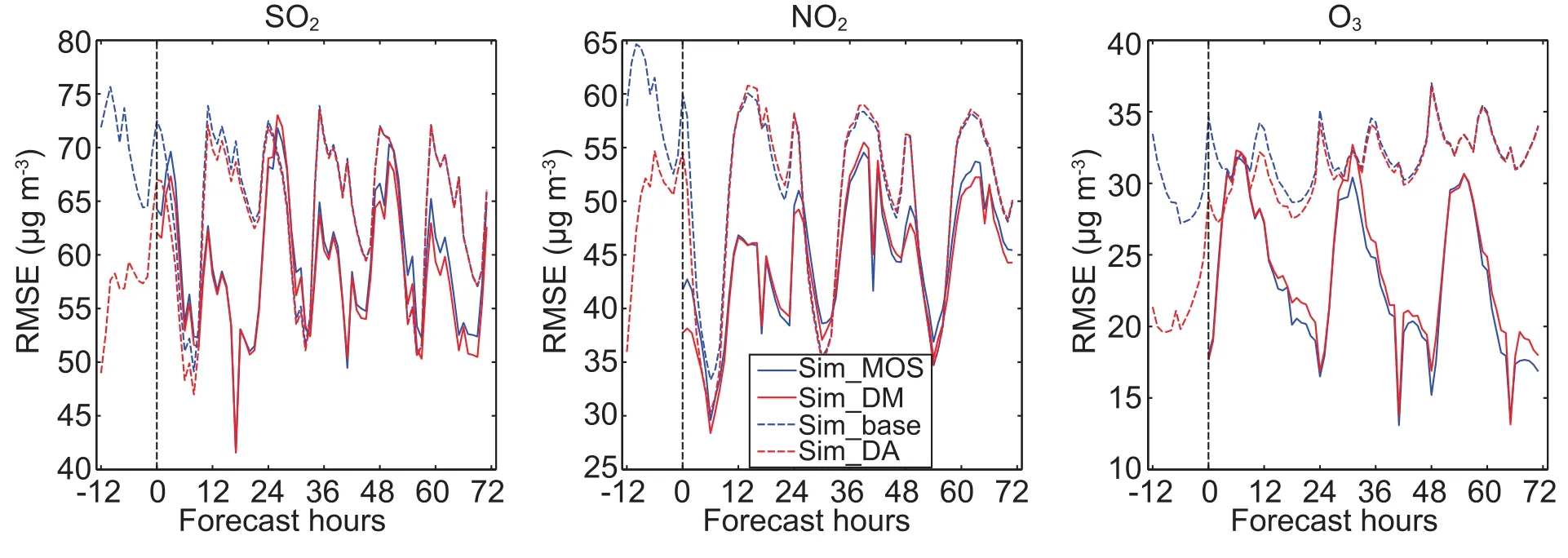
Fig.10.RMSE of three species at different forecast hours from ?12 h to 72 h from the same four experiments with solely emissions perturbed.

The forecast solely with MOS(SimMOS)performed better than that solely with 3DVar DA of CICs(SimDA).Such superiority of MOS could also be seen in all five species.That is,the implementation of MOS rather than 3DVar DA on CICs is more suitable for the aim of improving the operational forecast ability.

Considering the randomness of the influence of DA on error consistency,it is not impossible that combined use of both techniques will sometimes yield a worse forecast than MOS only.The potential degradation,which is expected to be mitigated by long-term averaging,should be considered,but is unlikely to concern forecasters because of the relatively limited difference yielded.However,considering the complexity of the two approaches,the feature of MOS,rather than DA of CICs,is recommended first when planning to improve your model forecast.

Given that refinement of the model grid is promising for additional forecast skill(Elbern et al.,2007),future work will concentrate on testing finer model grids in the vertical and horizontal dimensions,as well as different 3DVar observation error setups,in order to improve the effect of DA on the forecast.Of particular interest are species like SO2and NO2,which are unsatisfactorily forecasted by models with 3DVar.Also,to see if the conclusions will be different,we intend to try different DA methods,such as 4DVar and inverse modeling,which are able to adjust model parameters and emissions,which work as control parameters in a successful forecast(Schmidt and Martin,2003;Dubovik et al.,2008).Finally,another line of research would be extending the experiment time to explore whether any long-term statistical properties exist when using the DA and MOS techniques together.

Acknowledgements.This work was supported by the State Key Research and Development Program(Grant Nos.2017YFC0209803,2016YFC0208504,2016YFC0203303and 2017YFC0210106)and the National Natural Science Foundation of China(Grant Nos.91544230,41575145,41621005 and 41275128).The Hebei Meteorological Bureau of China is also thanked for making available the pollution monitoring data.

APPENDIX

Assume we have a systemxthat varies with timet,andxat timetis almost the same asxat timet?1 expect for a random errorw.Then,this system can be described by a system equation such as

For the systemx,assume we have some kind of measurementythat measuresxwith a random errorv.Then,we can write the measurement equation as

Ifwandvare both white noise,with their covariance already known asWandVand independent of each other,then we can obtain the best estimate ofxusing the following equations:

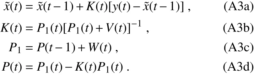
In these equations,?x(t)stands for the best estimate of the real systemx(t),which is usually unknown;andK(t)andP(t)are both intermediate variables whose meanings are not important.To complete a single one-dimensional Kalman filter iteration,the inputs of the equations areP(t?1)and?x(t?1)from the previous calculation,as well as a newly obtained measurementy(t).Then,the equations will yield newP(t)and?x(t),which will be saved for the next iteration.A detailed deduction of Eq.(A3)is beyond the scope of this work;interested readers should instead refer to Kalman(1960).

Here,three sequences of O3concentrations at 1200 UTC from three days’model output will be taken as an example to show the detailed steps of completing one iteration of MOS.It is assumed that on dayt(here,trepresents “today”),the following variables had been prepared:observation sequenceOi:i=1,2,···,tfrom the ground station;model 24-h forecast sequence and its correctionfi,24:i=1,2,···,t+1 and ?fi,24:i=1,2,···,t;model 48-h forecast sequence and its correctionandmodel 72-h forecast sequence and its correctionand:i=1,2,···,t+2(model forecast sequence can be obtained by interpolating the 3D field of the model output to the position of the site);as well as all thePand?xfrom the previous iteration.What we want is to generatefrom all variables above.

To obtaintwo different approaches will be applied simultaneously.In one approach,which is the same as in G02,x(i)=Oi?fi,24:i=1,2,···,tand1,2,···,tin Eqs.(A2)and(A3),so this approach is called the “difference approach”hereafter.v(i)in Eq.(A3)is set to zero to assume no measurement error,which meansVin Eq.(A3b)equals zero and the estimation ofWwould be unnecessary here.The calculation of Eq.(A3a)to Eq.(A3b)gives thethen,we assumexandThe subscript“d”means the corrected result from the difference approach.Additionally,we add another approach called the “ratio approach”.In this approach,all formulas are the same except(i)=Oi/fi,24:i=1,2,···,t,y(i)=Oi/fi,24:i=1,2,···,tandwhere the subscript“r”means the ratio approach.The final resultwill be chosen fromaccording to the method described in the final paragraph of this appendix.

Withobtained,it is now possible to calculatewe still carry out the calculation via two approaches:the difference and ratio approach.Now,andy(i)So,to some extent,works as a “measurement”of the real observationOi,or a“proxy”of observation as in section 2.2.At this time,v(i)cannot be set to zero in Eq.(A3)and the evaluation ofVandWbecomes necessary in completing the iteration.The estimation ofWandVresembles G02,in which

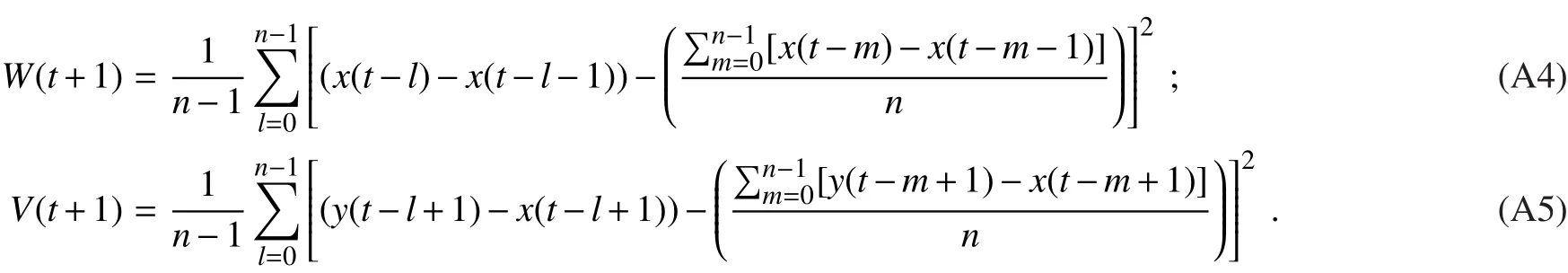
The variablenin Eqs.(A4)and(A5)is the number of sequence members participating in the statistics.A value from 7 to 9 is enough fornto generate a fairly good MOS effect,which means historical data from the past 7–9 days’observations and model output works as the virtual training sample for MOS.After completing the calculation of Eq.(A3a)–(A3d),?x(t+1)will be obtained and then?x(t+2)andcan be produced by replicating the process from the paragraph above.Another ratio approach is also performed to generateis chosen fromin the same way described in the final paragraph.

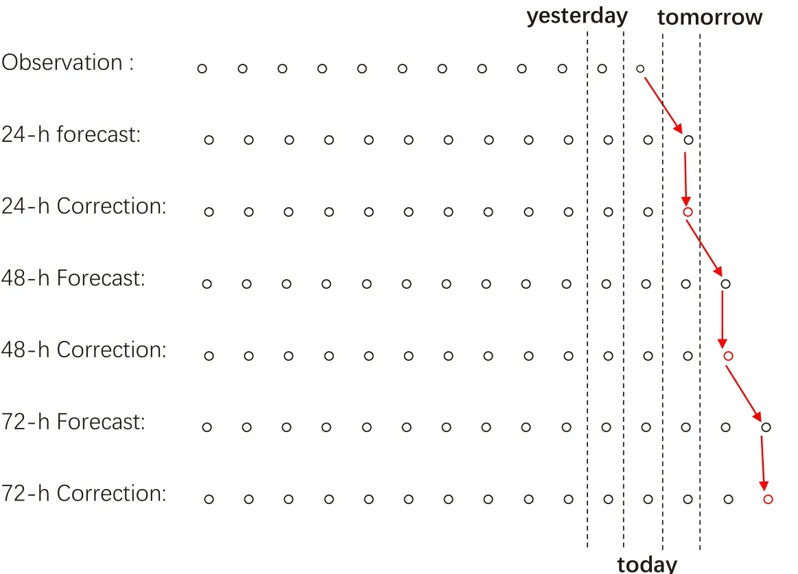
Fig.A1.Steps in applying the one-dimensional Kalman filter to correction over the whole 72 hours forecast period.The circles from left to right stand for values at the same hour from different days.Black circles are those existing before today’s calculation,while red ones are those generated from the calculation of today.

Fromto obtainingwhat has to be done is almost the same as fromThe differences mainly lie in some of the formulations.Taking the difference approach as an example,x(i)=Oi?fi,72:i=1,2,···,t,and the estimation ofVandWis changed to

Figure A1 is a schematic diagram showing how the algorithm described above is carried out,step by step.

The final output should be chosen from the difference and ratio approach according to their reasonability.From our experience,the difference approach tends to occasionally yield unreasonably low values,while the ratio approach sometimes gives results that are too high.Fortunately,the two conditions never happen simultaneously,and therefore the final output is from the ratio approach when its result is not too high(lower than the yearly averaged value of the species,for example).In cases where the ratio approach appears too high,the difference approach should be used instead.

REFERENCES

Ackermann,I.J.,H.Hass,M.Memmesheimer,A.Ebel,F.S.Binkowski,and U.Shankar,1998:Modal aerosol dynamics model for Europe:Development and first applications.Atmos.Environ.,32,2981–2999,http://dx.doi.org/10.1016/S1352-2310(98)00006-5.

Alexe,M.,and Coauthors,2015:Inverse modelling of CH4emissions for 2010–2011 using different satellite retrieval products from GOSAT and SCIAMACHY.Atmos.Chem.Phys.,15,113–133,http://dx.doi.org/10.5194/acp-15-113-2015.

Anadranistakis,M.,K.Lagouvardos,V.Kotroni,and H.Elefteriadis,2004:Correcting temperature and humidity forecasts using Kalman filtering:Potential for agricultural protection in Northern Greece.Atmos.Res.,71,115–125,http://dx.doi.org/10.1016/j.atmosres.2004.03.007.

Barbu,A.L.,A.J.Segers,M.Schaap,A.W.Heemink,and P.J.H.Builtjes,2009:A multi-component data assimilation experiment directed to sulphur dioxide and sulphate over Europe.Atmos.Environ.,43,1622–1631,http://dx.doi.org/10.1016/j.atmosenv.2008.12.005.

Barret,B.,and Coauthors,2008:Transport pathways of CO in the African upper troposphere during the monsoon season:A study based upon the assimilation of spaceborne observations.Atmos.Chem.Phys.,8,3231–3246,http://dx.doi.org/10.5194/acp-8-3231-2008.

Benedetti,A.,and Coauthors,2009:Aerosol analysis and forecast in the European Centre for Medium-Range Weather Forecasts Integrated Forecast System:2.Data assimilation.J.Geophys.Res.,114,D13205,http://dx.doi.org/10.1029/2008JD011115.

Bocquet,M.,and Coauthors,2015:Data assimilation in atmospheric chemistry models:Current status and future prospects for coupled chemistry meteorology models.Atmos.Chem.Phys.,15,5325–5358,http://dx.doi.org/10.5194/acp-15-5325-2015.

Denby,B.,M.Schaap,A.Segers,P.Builtjes,and J.Hor′alek,2008:Comparison of two data assimilation methods for assessing PM10exceedances on the European scale.Atmos.Environ.,42,7122–7134,http://dx.doi.org/10.1016/j.atmosenv.2008.05.058.

Dubovik,O.,T.Lapyonok,Y.J.Kaufman,M.Chin,P.Ginoux,R.A.Kahn,and A.Sinyuk,2008:Retrieving global aerosol sources from satellites using inverse modeling.Atmos.Chem.Phys.,8,209–250,http://dx.doi.org/10.5194/acp-8-209-2008.

Elbern,H.,A.Strunk,H.Schmidt,and O.Talagrand,2007:Emission rate and chemical state estimation by 4-dimensional variational inversion.Atmos.Chem.Phys.,7,3749–3769,http://dx.doi.org/10.5194/acp-7-3749-2007.

Galanis,G.,and M.Anadranistakis,2002:A one-dimensional Kalman filter for the correction of near surface temperature forecasts.Meteorological Applications,9,437–441,http://dx.doi.org/10.1017/S1350482702004061.

Geer,A.J.,and Coauthors,2006:The ASSET in tercomparison of ozoneanalyses:Method and first results.Atmos.Chem.Phys.,6,5445–5474,http://dx.doi.org/10.5194/acp-6-5445-2006.

Glahn,H.R.,and D.A.Lowry,1972:The use of model output statistics(MOS)in objective weather forecasting.J.Appl.Meteor.,11,1203–1211,http://dx.doi.org/10.1175/1520-0450(1972)011＜1203:TUOMOS＞2.0.CO;2.

Grell,G.A.,S.E.Peckham,R.Schmitz,S.A.McKeen,G.Frost,W.C.Skamarock,and B.Eder,2005:Fully coupled “online”chemistry within the WRF model.Atmos.Environ.,39,6957–6975,http://dx.doi.org/10.1016/j.atmosenv.2005.04.027.

Henze,D.K.,J.H.Seinfeld,and D.T.Shindell,2009:Inverse modeling and mapping US air quality in fluences of inorganic PM2.5 precursor emissions using the adjoint of GEOSChem.Atmos.Chem.Phys.,9,5877–5903,http://dx.doi.org/10.5194/acp-9-5877-2009.

Honore,C.,and Coauthors,2008:Predictability of European air quality:Assessment of 3 years of operational forecasts and analyses by the PREV’AIR system.J.Geophys.Res.,113,http://dx.doi.org/10.1029/2007JD008761.

Inness,A.,and Coauthors,2015:Data assimilation of satelliteretrieved ozone,carbon monoxide and nitrogen dioxide with ECMWF’s Composition-IFS.Atmos.Chem.Phys.,15,5275–5303,http://dx.doi.org/10.5194/acp-15-5275-2015.

Jiang,Z.Q.,Z.Q.Liu,T.J.Wang,C.S.Schwartz,H.C.Lin,and F.Jiang,2013:Probing into the impact of 3DVAR assimilation of surface PM10 observations over China using process analysis.J.Geophys.Res.,118,6738–6749,http://dx.doi.org/10.1002/jgrd.50495.

Kalman,R.E.,1960:A new approach to linear filtering and prediction problems.Journal of Basic Engineering,82,35–45,http://dx.doi.org/10.1115/1.3662552.

Li,Z.,Z.Zang,Q.B.Li,Y.Chao,D.Chen,Z.Ye,Y.Liu,and K.N.Liou,2013:A three-dimensional variational data assimila-tion system for multiple aerosol species with WRF/Chem and an application to PM2.5 prediction.Atmos.Chem.Phys.,13,4265–4278,http://dx.doi.org/10.5194/acp-13-4265-2013.

Libonati,R.,I.Trigo,and C.C.Dacamara,2008:Correction of 2m-temperature forecasts using Kalman Filtering technique.Atmos.Res.,87,183–197,http://dx.doi.org/10.1016/j.atmosres.2007.08.006.

Liu,Z.Q.,Q.H.Liu,H.C.Lin,C.S.Schwartz,Y.H.Lee,and T.J.Wang,2011:Three-dimensional variational assimilation of MODIS aerosol optical depth:Implementation and application to a dust storm over East Asia.J.Geophys.Res.,116,D23206,http://dx.doi.org/10.1029/2011JD016159.

Makar,P.A.,and Coauthors,2015:Feedbacks between air pollution and weather,Part 1:Effects on weather.Atmos.Environ.,115,442–469,http://dx.doi.org/10.1016/j.atmosenv.2014.12.003.

Mizzi,A.P.,A.F.Arellano Jr.,D.P.Edwards,J.L.Anderson,and G.G.P fister,2016:Assimilating compact phase space retrievals of atmospheric composition with WRF-Chem/DART:Aregional chemical transport/ensembleKalman filterdataassimilation system.Geoscientific Model Development,9,965–978,http://dx.doi.org/10.5194/gmd-9-965-2016.

Parrish,D.F.,and J.C.Derber,1992:The National Meteorological Center’s spectral statistical-interpolation analysis system.Mon.Wea.Rev.,120,1747–1763,https://doi.org/10.1175/1520-0493(1992)120＜1747:TNMCSS＞2.0.CO;2.

Saide,P.E.,G.R.Carmichael,S.N.Spak,P.Minnis,and J.K.Ayers,2012:Improving aerosol distributions below clouds by assimilating satellite-retrieved cloud droplet number.Proceedings of the National Academy of Sciences of the United States of America,109,11 939–11 943,http://dx.doi.org/10.1073/pnas.1205877109.

Saide,P.E.,and Coauthors,2015:Central American biomass burning smoke can increase tornado severity in the U.S.Geophys.Res.Lett.,42,956–965,http://dx.doi.org/10.1002/2014GL062826.

Schell,B.,I.J.Ackermann,H.Hass,F.S.Binkowski,and A.Ebel,2001:Modeling the formation of secondary organic aerosol within a comprehensive air quality model system.J.Geophys.Res.,106,28 275–28 293,http://dx.doi.org/10.1029/2001JD000384.

Schmidt,H.,and D.Martin,2003:Adjoint sensitivity of episodic ozone in the Paris area to emissions on the continental scale.J.Geophys.Res.,108,8561,http://dx.doi.org/10.1029/2001JD001583.

Schwartz,C.S.,Z.Q.Liu,H.C.Lin,and S.A.McKeen,2012:Simultaneous three-dimensional variational assimilation of surface fine particulate matter and MODIS aerosol optical depth.J.Geophys.Res.,117,D13202,http://dx.doi.org/10.1029/2011JD017383.

Semane,N.,and Coauthors,2009:On the extraction of wind information from the assimilation of ozone pro files in M′et′eo-France 4-D-Var operational NWP suite.Atmos.Chem.Phys.,9,4855–4867,http://dx.doi.org/10.5194/acp-9-4855-2009.

Stock well,W.R.,P.Middleton,J.S.Chang,and X.Y.Tang,1990:The second generation regional acid deposition model chemical mechanism for regional air quality modeling.J.Geophys.Res.,95,16 343–16 367,http://onlinelibrary.wiley.com/doi/10.1029/JD095iD10p16343/full.

Struzewska,J.,J.W.Kaminski,and M.Je fimow,2016:Application of model output statistics to the GEM-AQ high resolution air quality forecast.Atmos.Res.,181,186–199,http://dx.doi.org/10.1016/j.atmosres.2016.06.012.

Tang,X.,J.Zhu,Z.F.Wang,and A.Gbaguidi,2011:Improvement of ozone forecast over Beijing based on ensemble Kalman filter with simultaneous adjustment of initial conditions and emissions.Atmos.Chem.Phys.,11,12 901–12 916,http://dx.doi.org/10.5194/acp-11-12901-2011.

Tang,X.,J.Zhu,Z.F.Wang,A.Gbaguidi,C.Y.Lin,J.Y.Xin,T.Song,and B.Hu,2016:Limitations of ozone data assimilation with adjustment of NOxemissions:Mixed effects on NO2forecasts over Beijing and surrounding areas.Atmos.Chem.Phys.,16,6395–6405,http://dx.doi.org/10.5194/acp-16-6395-2016.

Taylor,A.A.,and L.M.Leslie,2005:A single-station approach to model output statistics temperature forecast error assessment.Wea.Forecasting,20,1006–1020,http://dx.doi.org/10.1175/WAF893.1.

van Loon,M.,and Coauthors,2007:Evaluation of long-term ozone simulations from seven regional air quality models and their ensemble.Atmos.Environ.,41,2083–2097,http://dx.doi.org/10.1016/j.atmosenv.2006.10.073.

Wang,Y.,K.N.Sartelet,M.Bocquet,and P.Chazette,2014:Modelling and assimilation of lidar signals over Greater Paris during the MEGAPOLI summer campaign.Atmos.Chem.Phys.,14,3511–3532,http://dx.doi.org/10.5194/acp-14-3511-2014.

Wargan,K.,S.Pawson,M.A.Olsen,J.C.Witte,A.R.Douglass,J.R.Ziemke,S.E.Strahan,and J.E.Nielsen,2015:The global structure of upper troposphere-lower stratosphere ozone in GEOS-5:A multiyear assimilation of EOS Aura data.J.Geophys.Res.,120,2013–2036,http://dx.doi.org/10.1002/2014JD022493.

Wilson,L.J.,and M.Vall′ee,2003:The Canadian Updateable Model Output Statistics(UMOS)system:Validation against perfect prog.Wea.Forecasting,18,288–302,http://dx.doi.org/10.1175/1520-0434(2003)018＜0288:TCUMOS＞2.0.CO;2.

Yerramilli,A.,and Coauthors,2010:Simulation of surface ozone pollution in the central gulf coast region using WRF/Chem model:Sensitivity to PBL and land surface physics.Advances in Meteorology,2010,Article ID 319138,http://dx.doi.org/10.1155/2010/319138.

Yin, X. M., T. Dai, N. A. J. Schutgens, D. Goto, T. Nakajima,and G. Y. Shi, 2016: Effects of data assimilation on the global aerosol key optical properties simulations.Atmos.Res.,178–179,175–186,https://doi.org/10.1016/j.atmosres.2016.03.016.

Yumimoto,K.,and Coauthors,2016:Aerosol data assimilation using data from Himawari-8,a next-generation geostationary meteorological satellite.Geophys.Res.Lett.,43,5886–5894,http://dx.doi.org/10.1002/2016GL069298.

Zhang,L.,and Coauthors,2015:Source attribution of particulate matter pollution over North China with the adjoint method.Environmental Research Letters,10,084011,https://doi.org/10.1088/1748-9326/10/8/084011.

Zhang,L.,and Coauthors,2016:Sources and processes affecting fine particulate matter pollution over North China:An adjoint analysis of the Beijing APEC Period.Environ.Sci.Technol.,50,8731–8740,http://dx.doi.org/10.1021/acs.est.6b03010.