
Large eddy simulation of free-surface flows*
2017-03-09 09:09:14RichardMcSherryKenChuaThorstenStoesser
水動力學(xué)研究與進(jìn)展 B輯 2017年1期
Richard J. McSherry, Ken V. Chua, Thorsten Stoesser
School of Engineering, Cardiff University, Cardiff, CF24 3AA, UK, E-mail: mcsherryr@cardiff.ac.uk
(Received January 10, 2017, Revised January 12, 2017)
Large eddy simulation of free-surface flows*
Richard J. McSherry, Ken V. Chua, Thorsten Stoesser
School of Engineering, Cardiff University, Cardiff, CF24 3AA, UK, E-mail: mcsherryr@cardiff.ac.uk
(Received January 10, 2017, Revised January 12, 2017)
This paper introduces and discusses numerical methods for free-surface flow simulations and applies a large eddy simulation (LES) based free-surface-resolved CFD method to a couple of flows of hydraulic engineering interest. The advantages, disadvantages and limitations of the various methods are discussed. The review prioritises interface capturing methods over interface tracking methods, as these have shown themselves to be more generally applicable to viscous flows of practical engineering interest, particularly when complex and rapidly changing surface topologies are encountered. Then, a LES solver that employs the level set method to capture free-surface deformation in 3-D flows is presented, as are results from two example calculations that concern complex low submergence turbulent flows over idealised roughness elements and bluff bodies. The results show that the method is capable of predicting very complex flows that are characterised by strong interactions between the bulk flow and the free-surface, and permits the identification of turbulent events and structures that would be very difficult to measure experimentally.
Large eddy simulation, free-surface, level set method, volume of fluid
Prof. Thorsten Stoesser is the Director of the Hydro-environmental Research Centre at Cardiff University. His main research interest is in developing advanced CFD tools and their application to hydraulic engineering and environmental fluid mechanics problems. Thorsten has published 100+ peer reviewed journal and conference papers on developing, testing and applying advanced CFD methods to predict hydrodynamics in rivers, estuaries and coastal waters, fluidstructure interaction of hydro turbines, and the nearfield dynamics of plumes and jets. He has co-authored the IAHR monograph “Large-eddy simulation in Hydraulics” and in 2012 and 2016 Dr. Stoesser received the American Society of Civil Engineers (ASCE) Karl Emil Hilgard Hydraulic Prize. In 2013, Prof. Stoesser won the International Association for Hydro-Environment Engineering and Research (IAHR) Harold Jan Shoemaker Award. His CFD group at Cardiff University currently consists of 8 Ph. D. students and 2 post-doctoral research associates, two of which have coauthored this feature article.

Introduction
The water surface is present in a wide range of flows that are of interest within engineering hydrodynamics, from the ubiquitous open channel flow to low submergence coastal flows past marine structures such as tidal stream turbines. Such surfaces, often termed “free-surfaces”, represent the boundary between the water body and the air above it, and may deform in response to the local flow physics including turbulence and bathymetric features. Deformation due to turbulence is generally small when compared to spatial and temporal variations of the mean surface position due to bed non-uniformity, ocean waves and the presence of hydraulic structures.
The equations governing free-surface flow aresignificantly more complex than those governing internal flow as they are subject to additional kinematic and dynamic boundary conditions at the (free) surface[1,2]. The kinematic condition is hyperbolic in nature and states that, since there can be no convective mass transfer across the air-water interface, the component of fluid velocity in the direction normal to the surface must be equal to the velocity of the surface itself. The dynamic boundary condition stipulates a force equilibrium at the interface, implying that the pressure and viscous forces exerted by the air and water respectively must balance. The boundary conditions introduce new nonlinear terms into the Navier Stokes equations, complicating their numerical solution significantly, although in hydraulics the dynamic condition is generally ignored since it is assumed that the surface tension can be neglected and the pressure on the air side can be assumed to be constant.
A number of novel approaches have been developed over the last thirty or so years to deal with the increased complexity introduced by the kinematic boundary condition; the interested reader is referred to Tsai and Yue[3]and Scardovelli and Zaleski[4]for indepth reviews of these developments. This paper focus on the application of free-surface modelling techniques within the framework of large eddy simulation (LES), a powerful eddy-resolving technique that is increasingly used to study complex turbulent flows in engineering scenarios[5]. The paper begins by presenting a concise overview of the numerical techniques that have been developed to deal with the free-surface problem by researchers working in diverse areas of engineering fluid dynamics. A numerical method that has been employed by the authors to compute freesurface flows in the field of environmental hydraulics is then presented. Finally results from two case studies involving low submergence open channel flow over (1) a rough bed and (2) a bed-mounted bluff body are presented and discussed.
1. Numerical methods for the computation of freesurface problems
There are various ways to handle the free-surface boundary in CFD. The easiest approach is to “ignore”free surface deformations and do the rigid lid approximation as will be described in Section 1.1. More complicated are numerical approaches that compute freesurface deformations as the numerical solution progresses (for instance at every time step) and these are largely grouped into two distinct categories: interface tracking methods and interface capturing methods (described in Sections 1.2 and 1.3, respectively).
1.1The rigid lid approximation
Within the field of hydraulics, the vast majority of simulations of flows involving water surfaces to date have employed the so-called rigid lid approximation, in which a fixed (generally flat) fixed surface or lid is used to represent the water surface. A free-slip boundary condition is stipulated at the lid, and the simulation is in fact that of a closed conduit with an artificial, frictionless condition at the lid. By definition the shear stress at the lid is zero, as is the component of the fluid velocity in the direction normal to it, but the pressure is free to vary as it would along a wall, which in turn produces zero shear stress there. This in effect constitutes a symmetry boundary condition. Rather than calculating the surface height with knowledge of the local fluid pressure, the problem is now reformulated and it is necessary to calculate the pressure based on the known height of the surface. The surface-elevation-gradient terms in the momentum equations for free-surface flows are thereby replaced by pressure gradients so that the dynamic effects of surface-elevation variations are properly accounted for by the rigid lid approximation method. The suppression of the actual surface deformation introduces an error in the continuity equation, but this is small when the surface deviation is small compared with the local water depth, say below 10% of the depth. Since local surface perturbations due to turbulence satisfy this condition in a large range of engineering flows the rigid lid approach has been applied with considerable success in a number of studies. This is particularly true of open-channel flows, where rigid lid LES and direct numerical simulations (DNS) have led to important insights on the structure of bed-generated turbulence[6-10].
To assess the validity of the rigid lid assumption Komori et al.[11]included the surface variations in their computation by including the kinematic boundary condition and compared the results with those from the rigid lid simulations of Lam and Banerjee[9]. They found that the free-surface deformations and near-surface normal velocities remained extremely small, leading them to conclude that the calculated flow behaviour near the free-surface did not differ from the rigid lid simulations. However it is expected that the errors will be more significant when the surface fluctuations are not small compared with the local water depth. In fact it is generally accepted that the rigid lid approximation is only strictly applicable to low Froude number (i.e.,Fr≤0.5) flows[12,13]. Kara et al.[14]performed two LES for flow through the same bridge contraction geometry, one with a rigid lid boundary and one with a free-surface capturing algorithm. The bulk Reynolds number was 27 200 and although the bulk Froude number was relatively low atFr= 0.37, locally values ofFr=0.78were reached as a result of the significant constriction imposed on the flow by the abutment (the ratio of channel width to abutment width was 3). Kara et al.’s results showedthat although the first order statistics and bed shear stresses were very similar for the two simulations, the instantaneous turbulence structure and second order statistics showed significant disparity. Their study highlighted the limitation of the rigid lid approximation and the requirement for more sophisticated approaches for the simulation of turbulent flows with complex water-surface deformations.
1.2Interface tracking methods
In interface tracking methods, also known as moving mesh methods, the mesh deforms after every time step to ensure that the boundary of the computational domain matches the free-surface position, thereby ensuring that the surface is explicitly tracked.
The principal advantages of interface tracking methods arise from the inherent reduction in the number of grid nodes since no nodes are required in the air phase, and the lack of numerical diffusion which tends to smooth out the interface in other methods[15]. Although the boundary integral technique is perhaps the interface tracking method that has attracted the most attention[16], due to its unsuitability to flows that are governed by the viscous Navier Stokes equations it is largely inapplicable to the field of hydraulics[17]. Much of the progress in interface tracking methods has been made in the field of ship hull hydrodynamics, where the key problem of interest is the interaction between the viscous boundary layer at the surface-piercing hull and the resulting surface wave[18,19]. Most studies have focused on achieving accurate predictions of this interaction using RANS approaches: in this context Nichols and Hirt[20], Farmer et al.[21]and Raven[22]employed free-surface height methods in which the freesurface was described as a height function, the solution of which was only loosely coupled temporally to the solution of the bulk pressure and velocities. Alessandrini and Delhommeau[23]on the other hand employed a similar method but solved the height function and bulk flow simultaneously. Van Brummelen et al.[24]and Raven and Van Brummelen[25]successfully applied an efficient iterative approach for steady and smooth surface waves, but noted that the performance of the method deteriorates and finally breaks down when steeper waves are simulated.
Miyata et al.[26]employed an interface tracking method using finite differences, with a sub-grid scale model for turbulent stresses, in simulations of flow past a ship hull in which the surface wave profile had reached a steady state, with Reynolds numbers ranging up to 105. Miyata et al.[27]improved the accuracy of the method by employing a similar approach with finite volumes, successfully simulating Reynolds numbers up to 106. In hydraulics an interface tracking method in the context of LES has been presented by Hodges and Street[28]who simulated the interaction of waves with a turbulent channel flow. These authors used an explicit time-discretization scheme to advance the free-surface by solving the kinematic boundary condition and solved a Poison-type equation after every time step to compute a new boundary-orthogonal grid. The Reynolds number in this case was relatively lowReτ=171so that the turbulent eddies and the surface deformations caused by them have rather large length and time scales. At Reynolds numbers of practical interest with much smaller turbulent length and time scales the recalculation of a new mesh would be extremely expensive. In fact, Hodges and Street state that in such cases their method is not suitable. In an attempt to avoid the creation of a new mesh after every time step Fulgosi et al.[29]used a mapping scheme that transfers the curvilinear physical space into an orthogonal coordinate system, employing the technique in a DNS of wind-sheared free-surface deformations.
A significant drawback of interface tracking methods concerns their ability to deal with complex surface topologies, especially in three dimensions and when singularities are observed. In general the methods fail beyond the time of the singularity and additional operations are required to remove individual nodes close to such features, thereby adding to the overall computational cost[15].
1.3Interface capturing methods
In interface capturing methods the water surface is not defined explicitly by the boundary of the numerical mesh as it is in interface tracking methods. Both fluid phases (i.e., water and air) are included on an Eulerian mesh, and an algorithm is therefore required to compute the evolution of the interface between them. In general interface capturing methods have the advantage of avoiding the grid surgery problem that is encountered in interface tracking methods, but common difficulties are how to maintain the thickness of the interface and conserve mass across it.
Harlow and Welch[30]first proposed the markerand-cell (MAC) method, in which massless particles are seeded in the water phase and are passively advected with the flow. An important advantage of the approach compared to most interface tracking methods arises from its ability to handle complex surface topologies such as breaking waves. The MAC method does however require a large number of seeded particles, making it relatively computationally expensive. As a result it has primarily been employed for 2-D or axis-symmetric flows[31-33], although more recently Tome et al.[34]and Sousa et al.[35]have extended it to three-dimensional tank filling and droplet splashing test cases. A comprehensive review of progress in MAC techniques can be found in McKee et al.[36].
Rather than representing the free-surface usingmarkers or particles, another class of interface capturing methods use scalar functions that do not need to coincide with grid lines and do not incur the vast computational expense of marker methods. The volume of fluid (VOF) method introduced by Hirt and Nichols[37]is one such approach. In this method the fraction of the liquid phase is determined by the solution of a transport equation for the void fractionF. By definitionFis unity in any cell that is fully submerged in the liquid, zero in any cell fully exposed in the gas, and some fraction in the range0<F<1in cells that contain the surface.
A number of research groups have proposed variants on Hirt and Nichols’ original method, generally with the intention of improving the robustness of the advection of the volume fraction and/or the accuracy of the geometrical representation of the surface; lower order schemes like first order upwinding tend to smear the interface due to numerical diffusion while high order methods suffer from stability issues and may result in numerical oscillations[38]. Existing variants include Hirt and Nichols’ original donor-acceptor scheme[37], the piecewise linear interface calculation method[39], the simple line interface calculation method (SLIC)[40], the flux-corrected transport method (FCT)[41], the compressive interface capturing scheme for arbitrary meshes (CICSAM)[42], and the intergamma compressive scheme[43]. The SLIC and PLIC methods, which both use geometric as opposed to algebraic interface reconstruction, have proved relatively popular since their introduction, in large part due to their relative simplicity and ability to deal with breaking and merging interfaces. Gopala and Van Wachem[38], however, state that SLIC suffers from high levels of numerical diffusion and limited accuracy, while PLIC is difficult to implement in three dimensions and to boundary-fitted grids. CICSAM and the inter-gamma method, on the other hand, are observed to conserve mass very well while also keeping the interface sharp, but they suffer from a high degree of sensitivity to the local Courant-Friedrichs-Lewy (CFL) number.
Despite the drawbacks of the VOF method, it has nonetheless grown in popularity since its introduction. Thomas et al.[44]proposed a novel method that combined the height function approach (Section 1.2) with VOF, achieving mass and momentum conservation with very little numerical dissipation. Although the method was capable of simulating arbitrarily large surface deformations the slope of the surface was subject to a limit related to the cell aspect ratio, and breaking wave simulations were therefore not permitted. The method was applied to turbulent flow in a straight open channel by Shi et al.[45]in a relatively poorly resolved LES that was designed to be run on a desktop workstation to demonstrate the applicability of the
The level-set method (LSM), which originated in computer graphics, has recently become a popular interface-capturing method for multi-phase flows. Like VOF, LSM employs a scalar function rather than Lagrangian particles, thereby circumventing the computational expense that hinders methods such as MAC. It was originally proposed by Osher and Sethian[55]and was developed for the computation and analysis of the motion of an interface between two fluid phases in two or three dimensions. In the LSM the interface is represented by the zero set of a smooth distance function,, that is defined for the entire physical domain. The conservation equations are solved for both liquid and gas phase and the interface is advected according to the local velocity vector.
The LSM method has proven a very versatile approach, capable of computing geometrically complex surfaces involving corners and cusps, and can deal with rapidly changing topologies robustly. Furthermore it can be generalised to three-dimensional problems relatively easily[15].
Withinthefieldofhydraulics,Yueetal.[56]emmethod within an engineering context. The turbulence metrics were found to be in agreement with experimental and DNS data.
Sanjou and Nezu[46]reported LES of turbulent free-surface flows past emergent vegetation in compound open channels. Although no details of the VOF scheme were given, the results demonstrated the applicability of surface capturing approaches to LES of complex flows in hydraulics.
Xie et al.[47]performed LES of turbulent openchannel flow over two-dimensional dunes. The simulations were designed to replicate the experiments of Polatel[48], and two LES were carried out, one with the rigid lid approximation and one in which the free-surface was modelled using CICSAM VOF. The bulk Reynolds number, based on mean depth and bulk flow velocity, was 28 000. The relative submergence, that is to say the ratio of flow depth to dune height, was 4 and the Froude number was relatively low at 0.32. The mean velocity profiles from both LES agreed well with the experimental data, but some discrepancies were observed in the turbulence statistics. Furthermore, the VOF simulation revealed the presence of some degree of surface renewal in the form of upwelling and drafts.
The ability of the VOF method to cope with complex surface topologies that involve breaking up and merging has naturally led to its application to the study of breaking waves. While a number of early studies addressed this problem using RANS approaches[49,50], relatively few LES have been performed, and most of those are restricted to two dimensions[51-53]. Christensen[54], however, extended into three dimensions but the simulations suffered from poor grid resolution.ployed the LSM in LES of turbulent open channel flow over fixed dunes. The relative submergence was 6.6 and therefore significantly higher than in the VOF study of Xie et al.[47]. It was observed that the method was able to accurately and realistically calculate the unsteady free-surface motion and also provided evidence of boils, upwelling and downdraft at the water surface. Suh et al.[57]report results from LES of flow past a vertical circular cylinder that protruded from the water surface. The LSM was used to capture the water surface dynamics and it was observed that the classic Karman-type vortex shedding is attenuated in the near-surface region, to be replaced by much smaller vortices. Kara et al.[58]performed LES of flow through a submerged bridge with overtopping, using LSM to capture the free-surface dynamics. The simulation revealed very complex flow phenomena, including a plunging nappe and standing wave at the surface downstream of the bridge, a horizontal recirculation in the wake of the lateral abutment and vertical recirculation created by the plunging flow. The simulation results agreed very well with complementary experimental measurements in terms of the water surface deformation. Kang and Sotiropoulos[59]performed a LES of open channel turbulent flow over a river restoration scheme, also using the LSM for the freesurface capture, on a curvilinear grid. Good agreement with experimental data was observed in terms of mean velocities and turbulence statistics, and the method was shown to be capable of capturing very complex flow dynamics downstream of the structure, including a standing wave that was characterised by very high levels of near-surface turbulence.
As mentioned earlier, a difficulty commonly associated with front capturing techniques is how to maintain the interface thickness while satisfying mass conservation. For the LSM, the specific problem is that, althoughshould remain a signed distance function at all times, advection due to the local velocity vector naturally acts to distort the function. The LSM overcomes this difficulty by using re-initialisation techniques, which involve resetting thefield at regular intervals, thereby ensuring that it remains a signed distance function with the same zero level set. The first of these reinitialisation techniques was proposed by Sussman et al.[60], with subsequent modifications developed by Peng et al.[61], Russo and Smereka[62]and Sussman and Puckett[63], among others. The reinitialisation can, however, result in numerical errors and the introduction of numerical oscillations in the free-surface[64].
In recent years a number of efforts have been made to improve the mass conservation properties of the LSM by coupling it with other techniques to form so-called hybrid methods. Enright et al.[65], for example, derived a particle level set method (PLSM) that used Lagrangian marker particles to reconstruct the interface in regions of poor resolution, finding that its mass conservation and interface resolution quantities were comparable to those of VOF and pure Lagrangian methods respectively. A hybrid method that has shown promise in recent years is the coupled level set volume of fluid (CLSVOF) method[66], which has been shown to perform better than the PLSM for simulations of practical engineering flows[67,68].
2. A two-phase LES solver with interface capturing
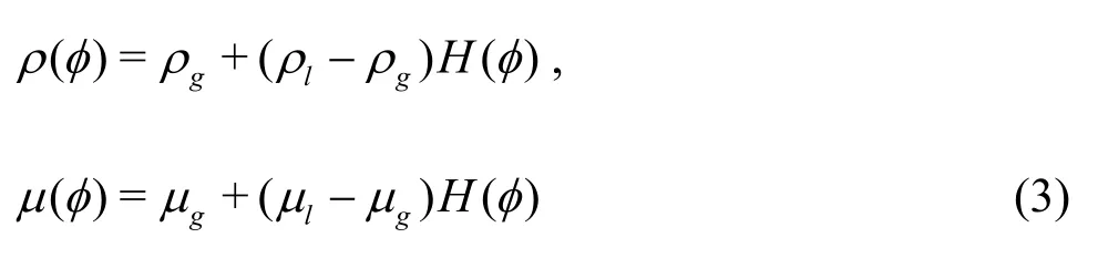
This section presents details of a numerical solver that has been used by the authors and co-workers for LES of open channel flows with complex free-surface interactions. The governing equations for an unsteady, incompressible, viscous flow of a Newtonian fluid are solved using the in-house code HYDRO3D[7,8,69-71]. An LES approach is employed to simulate directly the large, energy carrying eddies while scales smaller than the grid size are accounted for using the WALE subgrid scale model[72]. The code is a refined and improved version of the open-channel LES code that was validated for flow over dunes[73], flow in compound channels[74]and flow in contact tanks[75,76]. HYDRO3D is based on finite differences with staggered storage of the Cartesian velocity components on uniform Cartesian grids. Second-order central differences are employed for the diffusive terms while convective fluxes in the momentum and level-set equations (see below) are approximated using a fifth-order weighted essentially non-oscillatory (WENO) scheme. The WENO scheme offers the necessary compromise between numerical accuracy and algorithm stability (especially important for the free-surface algorithm, see below). A fractional-step method is used with a Runge-Kutta predictor and the solution of a pressurecorrection equation in the final step as a corrector. A multi-grid method is employed to solve the Poisson equation. The code is parallelized via domain decomposition, and the standard message passing interface (MPI) accomplishes communication between sub-domains.
The free-surface is captured using the level set method (LSM) developed by Osher and Sethian[55]. As explained in Section 1.3, the LSM employs a level set signed distance function,, which has zero value at the phase interface and is negative in air and positive in water. This method is formulated as:
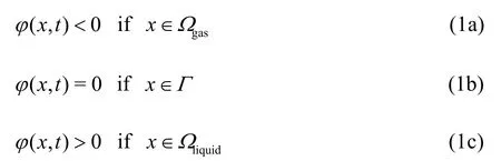
where?gasand?liquidrepresent the fluid domains for gas and liquid, respectively, andis the interface. The interface moves with the fluid particles, expressed through a pure advection equation of the form
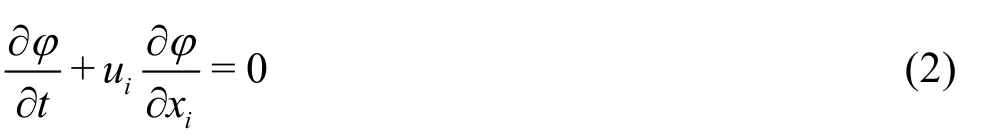
where
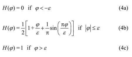
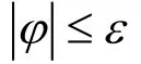
The LSM has proven successful in the description of complex multi-phase boundaries and it gives continues approximations[79,80,59]. On the other hand, the LSM is known to have difficulties in conserving mass for strongly distorted interfaces due to numerical dissipation introduced in the discretization of Eq.(2) when using upwind biased schemes. Because this is a pure advection problem, central differencing schemes are unstable[81]. To minimize numerical dissipation, a fifth-order WENO scheme[80]is used. Another difficulty with LSM is thatdoes not maintain its property ofas time proceeds. To overcome this problem, a re-initialization technique introduced by Sussman et al.[60]is employed, which also helps in improving mass conservation issues. The re-initialized signed distance functionis obtained by solving the partial differential equation given by[60]

whered0(x,0)=?(x,t),tais the artificial time ands(d0)is the smoothed signed function given as
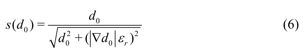
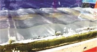
Fig.1(a) Experimental set-up
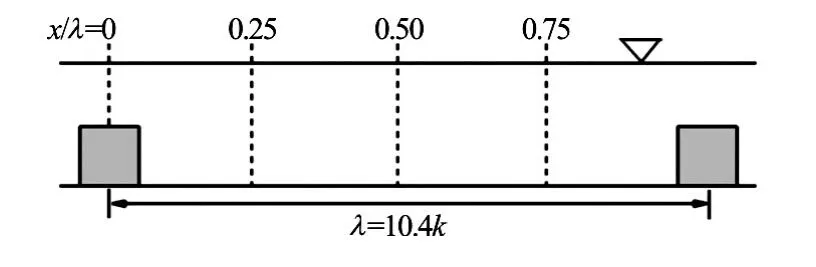
Fig.1(b) Schematic showing flow configuration
3. Example calculations
3.1Low submergence flow over transverse square bars
The first test case concerns low submergence turbulent flow over bed-mounted transverse square bars in an open channel. The case is one of six that were investigated experimentally in a 10 m long, 0.3 m wide glass-walled recirculating flume in the Hyder Hydraulics Laboratory at Cardiff University[82]. A series of plastic square bars of width 0.3 m and crosssection 12 mm×12 mm were installed along the length of the flume, perpendicular to the direction of mean flow (Fig.1(a)). The roughness height,k, was therefore 12 mm. Two different bar spacings were investigated: the case that has been selected for presentation here had a bar spacing ofλ=125 mm, corresponding to a normalised spacing ofλ/k=10.4(Fig.1(b))which, according to Coleman et al.[83], constitutes k-type roughness. The bed slope was fixed at 1:50 and the flow rate was 2.5 l/s. The relative submergence,H/k, whereHis the double-averaged height of the free-surface above the channel bed, was 2.8. Measurements of instantaneous velocity and free-surface position were taken in a section of the flume where the flow was considered to be uniform and fully-developed. The flow was also considered to be spatially periodic with wavelengthλin the streamwise direction, that is to say the temporal mean values of all flow variables in successive cavities between bars were considered to be the same. The bulk Reynolds number was 8 300 and the friction Reynolds numberReτ(=u?H/v)whereu?is the global shear velocity based on the bed shear stress,τ, was 2 800. The global Froude number of the flow,Fr=(Ub/gH), was 0.72 but local values based on local depths and velocities varied significantly from this global value.
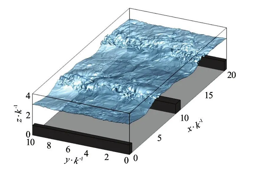
Fig2(a) Computational domain, including instantaneous water surface
Figure 2(a) presents the computational domain that was used for the simulation, along with an isosurface representing the position of the simulated water surface at an arbitrary moment in time. The domain spanned two cavities in the streamwise direction and the dom ain d imensions were 20.8k×10k×4.2 5k. The domain was discretised with a uniform grid and the number of grid points was 1 024×512×408 (= 2.14×10⁸) points. The grid spacing in wall units, using the global shear velocity for normalisation, was as follows:Δx+=21.8,Δy+=20.9and Δz+=11.1. Figure 2(a) shows that the domain extended higher than the free-surface: the volume above the surface was occupied by the air phase, and the volume below was occupied by the water phase. A free-slip boundary condition was applied to the top of the domain while a no-slip condition was stipulated on the channel bed. The bars were represented by immersed boundaries, which achieve an effective no-slip boundary condition on their surfaces[84]. Periodic boundary conditions were applied at the streamwise and spanwise boundaries, and the flow was driven by the component of gravitational acceleration acting parallel to the channel bed, based on the bed slope that was applied in the flume experiment (1:50). The global shear velocity in the simulation was therefore exactly the same as in the experiment.
The simulation was initiated with a planar rigid lid applied at the mean free-surface position that was recorded in the experiments. A free-slip boundary condition was stipulated at the rigid lid and the simulation was run for 100 000 time steps, which corresponded to approximately 8 flow through periods,Tf(=Lx/Ub, whereLxis the length of the domain), to allow the flow to develop fully. The simulation was then restarted without the rigid lid but with the level set algorithm now activated to track the free-surface. Averaging of the flow quantities began after 2 more flow through periods, and continued for 10 further flow through periods to ensure that the turbulence statistics were well converged. Further averaging was performed in the homogeneous spanwise direction to obtain a smooth distribution of turbulence statistics. Figures 2(a) and 2(b) show that the flow is characterised by dramatic and dynamic surface deformation, resulting in a standing wave in the cavity between bars. Figure 2(b), which is a close-up of the surface at one of the standing waves, gives an indication of the level of resolution that was achieved in the simulation. As seen from this figure, the standing waves are superimposed by smaller deflections and disturbances which are the result of the turbulence underneath the water surface.
Figure 3 presents contours of normalised streamwise velocity,u/Ub, at an arbitrary moment in time on the mid-plane of the domain. The position of the water surface at this moment in time has also been included for reference. Significant flow acceleration is observed above the bars, accompanied by a corresponding c ont raction of the sur face. V ery stro ng rec irculationsareobservedinthewakesofthebars,withreattachment to the bed taking place between a quarter and half way downstream of each bar. Downstream of the recirculation area the flow decelerates markedly, the water surface reacts rapidly and this entails the standing wave, which moves backwards and forwards probably in sync with the size of the local recirculation zone behind each bar.
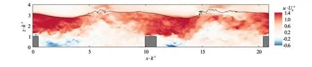
Fig.3 Contours of normalised streamwise velocity in the mid-plane of the domain. Solid black line indicates location of the water surface
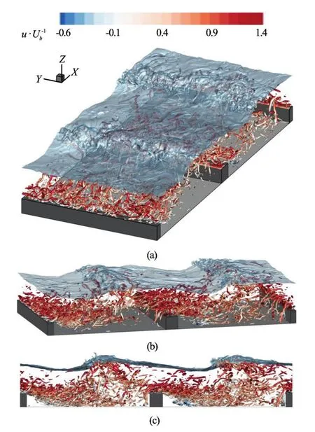
Fig.4 Iso-contours ofQ-criterion and water surface from three different perspectives
Figures 4(a)-(c) present views ofQ-criterion iso-surfaces at the same moment in time, from different perspectives. The corresponding free-surface is also plotted. Figure 4(a) reveals that fairly large spanwise vortices, the width of which are approximately one third of the local flow depth, are generated at the roughness tops. These vortices then stretch and deform into hairpin-type vortices soon after they are shed. Figures 4(b) and (c) reveal that most of the coherent turbulence is generated at the bars and these are advected by the flow downstream and in the lower half of the water column, just above the recirculation zone. The flow and turbulence structures reattach in the cavity between the bars and the vortices are lifted upwards towards the water surface. In Fig.4(c) significant interaction is observed at the standing wave, which is characterised by a periodic instability and the production of small-scale spanwise vortices. Some merging of the surface-generated turbulence with that generated at the bed is observed immediately downstream of the standing wave.
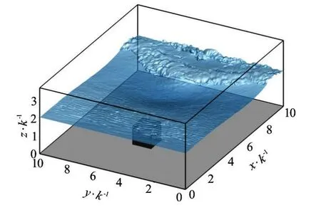
Fig.5 Computational domain showing location of bed-mounted cube and instantaneous water surface
3.2Low submergence flow over a bed-mounted cube
The second test case is a shallow flow over a cube mounted on the bed of an open channel. The case is based on the wind tunnel experiments of Martinuzzi[85]and Martinuzzi and Tropea[86]and their data is used to validate the LES in the first instance. In the experiments the cube was mounted on the lower wall and occupied half of the tunnel height, i.e.,Hw/k=2, whereHwis the wind tunnel height andkis the cube height. The Reynolds number of the flow based on bulk velocity and cube height wasRe=40 000and the flow was deemed to be fully developed in the section in which the cube was placed. After successful validation (not shown for brevity), the upper fixed wall (of the tunnel) was replaced by a free water surface initially placed at a heightH=2k, such that therelative submergence wasH/k=2, and the Reynolds number based on water depth and bulk velocity was kept atRe=40 000. The global Froude number was 0.6. Figure 5 presents the computational domain that was employed: it extended3kupstream,4klaterally and7kdownstream of the cube centre. In the vertical direction the domain extended3.5kabove the bed, with the top1.5koccupied by the air phase. The domain was discretised by a uniform grid with 600× 384×300 (= 69×106) grid points. The cube was represented by immersed boundaries.
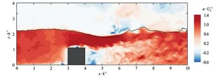
Fig.6 Contours of normalised streamwise velocity in the mid-plane of the domain (i.e., cube centreline). Solid black line indicates location of the water surface
Fully developed turbulent flow was applied at the inflow boundary: this was achieved by performing a precursor simulation of turbulent open channel flow with periodic streamwise boundary conditions. When the flow in this precursor simulation was judged to be fully developed it was continued for a further 10 000 time steps and the 2-D instantaneous flow field from the outflow plane was saved at every time step. This produced 10 000 2-D planes of instantaneous turbulent flow which were applied at successive time steps at the inflow boundary of the cube simulation in a cyclical manner, thereby ensuring a continuous fullydeveloped turbulent inflow for the duration of the simulation. Convective and periodic conditions were stipulated at the outflow and lateral boundaries respectively, while a no-slip condition was applied on the channel bed.
Figure 6 presents contours of instantaneous normalised streamwise velocity at an arbitrary moment in time, on the mid plane of the domain. The position of the water surface is included for reference. The water surface experiences a notable dip immediately downstream of the cube, and this is due to the significant local acceleration in the upper part of the water column and a strong recirculating region in the cube wake. In a similar manner to the flow over bars, the flow decelerates markedly downstream of the recirculation zone and causes a standing wave, above the reattachment zone.
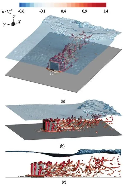
Fig.7 Iso-contours ofQ-criterion and water surface from three different perspectives
Figures 7(a)-7(c) present views ofQ-criterion iso-surfaces at the same moment in time, from different perspectives, as well as an iso-surface of the instantaneous water surface. The standing wave that manifests downstream of the cube displays a pronounced bow shape, owing to the three-dimensionality of the submerged obstacle. The wave appears to break further downstream away from the centreline and the minimum water level is found in the centreline of the channel and approximately1.5kdownstream of the cube. In terms of turbulent flow structures, there is a well-defined horseshoe vortex upstream of the cube aswell as an arch vortex that is generated at the leading edge of the cube, breaks into vertical vortices sideways of the cube and a horizontal roller-type vortex on the top of the cube. All three vortices are being convected by the flow into the downstream area of the cube. Figure 7(b) shows that the roller vortex deforms and appears as hairpin-type vortices in the cube wake. Figure 7(c) highlights the dip in the water surface downstream of the cube, and suggests that the turbulent structures generated by the cube eventually travel upwards towards the surface, downstream of the standing wave. In contrast to the flow over the bars, the most coherent turbulence structures do not appear to be directly interacting with the standing wave.
4. Conclusions
A review of numerical methods for free-surface flow simulation and their applications to flows of engineering interest has been undertaken, with particular emphasis on LES. The advantages, disadvantages and limitations of the various methods have been discussed. In general interface capturing methods, particularly VOF and LSM, appear to be more suitable and hence prevalent in terms of application to engineering flows, especially those involving complex water surface deformations. Recently these have been implemented and used successfully within the framework of LES and this combination has proven a powerful tool to reveal complex turbulence enhanced water surface displacements.
Further, a LES-based solver that employs the Level Set Method to capture free-surface deformation in 3-D flows has been presented, as have results from two example calculations that concern complex low submergence turbulent flows over idealised roughness elements and bluff bodies. The results give a good indication that the method is capable of predicting very complex flows that are characterised by strong interactions between the bulk flow and the free-surface, and permits the identification of turbulent structures and events that would be very difficult to achieve experimentally.
Acknowledgements
This work was supported by the UK Engineering and Physical Sciences Research Council (EPSRC). The computations presented in the paper were carried out on Cardiff University’s supercomputer Raven, hosted by Advanced Research Computing @ Cardiff (ARCCA), and High Performance Computing Wales’Cardiff Hub.
[1] Hodges B. R., Street R. L. On simulation of turbulent nonlinear free-surface flows [J].Journal of Computational Physics, 1999, 151(2): 425-457.
[2] Ferziger J. H., Peric M. Computational methods for fluid dynamics [M]. 3rd edition. Berlin, Germany: Springer, 2002.
[3] Tsai W., Yue D. K. P. Computation of nonlinear free-surface flows [J].Annual Review of Fluid Mechanics, 1996, 28(1): 249-278.
[4] Scardovelli R., Zaleski S. Direct numerical simulation of free-surface and interfacial flow [J].Annual Review of Fluid Mechanics, 1999, 31(1): 567-603.
[5] Stoesser T. Large-eddy simulation in hydraulics: Quo Vadis? [J].Journal of Hydraulic Research, 2014, 52(4): 441-452.
[6] Singh K. M., Sandham N. D., Williams J. J. R. Numerical simulation of flow over a rough bed [J].Journal of Hydraulic Engineering, ASCE, 2007, 133(4): 386-398.
[7] Stoesser T., Nikora V. I. Flow structure over square bars at intermediate submergence: Large eddy simulation study of bar spacing effect [J].Acta Geophysica, 2008, 56(3): 876-893.
[8] Bomminayuni S., Stoesser T. Turbulence statistics of openchannel flow over a rough bed [J].Journal of Hydraulic Engineering, ASCE, 2011, 137(11): 1347-1358.
[9] Lam K., Banerjee S. On the condition of streak formation in a bounded turbulent flow [J].Physics of Fluids A-Fluid Dynamics, 1992, 4(2): 306-326.
[10] Pan Y., Banerjee S. A numerical study of free-surface turbulence in channel flow [J].Physics of Fluids, 1995, 7(7): 1649-1664.
[11] Komori S., Nagaosa R., Murakami Y. et al. Direct numerical simulation of three-dimensional open-channel flow with zero-shear gas–liquid interface [J].Physics of Fluids A–Fluid Dynamics, 1993, 5(1): 115-125.
[12] Koken M., Constantinescu G. An investigation of the dynamics of coherent structures in a turbulent channel flow with a vertical sidewall obstruction [J].Physics of Fluids, 2009, 21(8): 085104.
[13] Paik J., Sotiropoulos F. Coherent structure dynamics upstream of a long rectangular block at the side of a large aspect ratio channel [J].Physics of Fluids, 2005, 17(11): 115104.
[14] Kara S., Kara M., Stoesser T. et al. Free-surface versus rigid-lid LES computations for bridge-abutment flow [J].Journal of Hydraulic Engineering, ASCE, 2015, 141(9): 04015019.
[15] Chang Y. C., Hou T. Y., Merriman B. et al. A level set formulation of eulerian interface capturing methods for incompressible fluid flows [J].Journal of Computational Physics, 1996, 124(2): 449-464.
[16] Hou T. Y., Lowengrub J. S., Shelley M. J. Removing the stiffness from interfacial flows with surface tension [J].Journal of Computational Physics, 1994, 114(2): 312-338.
[17] Hou T. Y., Lowengrub J. S., Shelley M. J. Boundary integral methods for multicomponent fluids and multiphase materials [J].Journal of Computational Physics, 2001, 169(2): 302-362.
[18] Toda Y., Stern F., Longo J. Mean-flow measurements in the boundary layer and wake field of a Series 60 CB = 0.6 ship model. Part 1: Froude numbers 0.16 and 0.316 [J].Journal of Ship Research, 1992, 36(4): 360-377.
[19] Longo J., Stern F., Toda Y. Mean-flow measurements in the boundary layer and wake field of a Series 60 CB = 0.6 ship model. Part 2: Scale effects on near field wave patterns and comparisons with inviscid theory [J].Journal of Ship Research, 1993, 37(1): 16-24.
[20] Nichols B. D., Hirt C. W. Calculating three-dimensional free surface flows in the vicinity of submerged and exposed structures [J].Journal of Computational Physics, 1973, 12(2): 234-246.
[21] Farmer J., Martinelli L., Jameson A. A fast multigrid method for the non-linear ship wave problem with a free surface [C].Proceedings of the Sixth International Conference on Numerical Ship Hydrodynamics. Iowa, USA, 1993, 155-172.
[22] Raven H. C. A solution method for the nonlinear ship wave resistance problem [D]. Doctoral Thesis, Delft, The Netherlands: Delft University of Technology, 1996.
[23] Alessandrini B., Delhommeau G. A multigrid velocitypressure free-surface-elevation fully coupled solver for calculation of turbulent incompressible flow around a hull [C].Proceedings of the 21th Symposium on Naval Hydrodynamics. Trondheim, Norway, 1996.
[24] Van Brummelen E. H., Raven H. C., Koren B. Efficient numerical solution of steady free-surface Navier-Stokes Flow [J].Journal of Computational Physics, 2001, 174: 120-137.
[25] Raven H., Van Brummelen E. A new approach to computing steady free-surface viscous flow problems [C].1st MARNET-CFD workshop. Barcelona, Spain, 1999.
[26] Miyata H., Toru S., Baba N. Difference solution of a viscous flow with free-surface wave about an advancing ship [J].Journal of Computational Physics, 1987, 72(2): 393-421.
[27] Miyata H., Zhu M., Wantanabe O. Numerical study on a viscous flow with free-surface waves about a ship in steady straight course by a finite-volume method [J].Journal of Ship Research, 1992, 36(4): 332-345.
[28] Hodges B. R., Street R. L. On simulation of turbulent nonlinear free-surface flows [J].Journal of Computational Physics, 1999, 151(2): 425-457.
[29] Fulgosi M., Lakehal D., Banerjee S. et al. Direct numerical simulation of turbulence in a sheared air-water flow with a deformable interface [J].Journal of Fluid Mechanics, 2003, 482: 319-345.
[30] Harlow F. H., Welch J. E. Numerical calculation of timedependent viscous incompressible flow of fluid with free surface [J].Physics of Fluids, 1965, 8(12): 2182.
[31] Viecelli J. A. A computing method for incompressible flows bounded by moving walls [J].Journal of Computational Physics, 1971, 8(1): 119-143.
[32] Veldman A. E. P., Vogels M. E. S. Axisymmetric liquid sloshing under low-gravity conditions [J].Acta Astronautica, 1984, 11(10-11): 641-649.
[33] Armenio V. An improved MAV method (SIMAC) for unsteady high-Reynolds free surface flows [J].International Journal for Numerical Methods in Fluids, 1997, 24(2): 185-214.
[34] Tome M. F., Filho A. C., Cuminato J. A. et al. GENSMAC3D: A numerical method for solving unsteady three-dimensional free surface flows [J].International Journal of Numerical Methods in Fluids, 2001, 37(7): 747-796.
[35] Sousa F. S., MangiavacchI N., Nonato L. G. et al. fronttracking/front-capturing method for the simulation of 3D multi-fluid flows with free surfaces [J].Journal of Computational Physics, 2004, 198(2): 469-499.
[36] McKee S., Tome M. F., Ferreira V. G. et al. The MAC method [J].Computers and Fluids, 2008, 37(8): 907-930.
[37] Hirt C. W., Nichols B. D. Volume of fluid (VOF) method for the dynamics of free boundaries [J].Journal of Computational Physics, 1981, 39(1): 201-225.
[38] Gopala V. R., Van Wachem B. G. M. Volume of fluid methods for immiscible-fluid and free-surface flows [J].Chemical Engineering Journal, 2008, 141(1): 204-221.
[39] Youngs D. L., Morton K. W., Baines M. J. Time-dependent multi-material flow with large fluid distortion (Numerical methods for fluid dynamics) [M]. New York, USA: Academic Press, 1982, 273-285.
[40] Noh W. F., Woodward P. SLIC (simple line interface calculations) [J].Lecture Notes in Physics, 1979, 59: 330-340.
[41] Boris J. P., Book D. L. Flux-corrected transport. I. SHASTA, a fluid transport algorithm that works [J].Journal of Computational Physics, 1973, 11(1): 38-69.
[42] Ubbink O. Numerical prediction of two fluid systems with sharp interfaces [D]. Doctoral Thesis, London, UK: Imperial College of Science, Technology and Medicine, 1997.
[43] Jasak H., Weller H. G. Interface-tracking capabilities of the inter-gamma differencing scheme [R]. Technical Report, London, UK: Imperial College, University of London, 1995.
[44] Thomas T. G., Leslie D. C., Williams J. J. R. Free-surface simulations using a conservative 3D code [J].Journal of Computational Physics, 1995, 116(1): 52-68.
[45] Shi J., Thomas T. G., Williams J. J. R. Free-surface effects in open channel flow at moderate Froude and Reynold’s numbers [J].Journal of Hydraulic Research, 2000, 38(6): 465-474.
[46] Sanjou M., Nezu I. Large eddy simulation of compound open-channel flows with emergent vegetation near the floodplain edge[C].9th International Conference on Hydrodynamics. Shanghai, China, 2010, 565-569.
[47] Xie Z., Lin B., Falconer R. A. Turbulence characteristics in free-surface flow over two-dimensional dunes [J].Journal of Hydro-Environment Research, 2014, 8(3): 200-209. [48] Polatel C. Large-scale roughness effect on free-surface and bulk flow characteristics in open-channel flows [D]. Doctoral Thesis. Iowa, USA: University of Iowa, 2006.
[49] Bradford S. F. Numerical simulation of surf zone dynamics [J].Journal of Waterway, Port, Coastal and Ocean Engineering, 2000, 126(1): 1-13.
[50] Bakhtyar R., Barry D. A., Li L. et al. Modeling sediment transport in the swash zone: A review [J].Ocean Engineering, 2009, 36(9-10), 767-783.
[51] Watanabe Y., Saeki H. Three-dimensional large eddy simulation of breaking waves [J].Coastal Engineering Journal, 1999, 41(3-4): 281-301.
[52] Watenabe Y., Saeki H. Velocity field after wave breaking [J].International Journal of Numerical Methods in Fluids, 2002, 39(7): 607-637.
[53] Lubin P., Glockner S., Kimmoun O. et al. Numerical study of the hydrodynamics of regular waves breaking over a sloping beach [J].European Journal of Mechanics B/Fluids, 2011, 30(6): 552-564.
[54] Christensen E. D. Large eddy simulation of spilling and plunging breakers [J].Coastal Engineering, 2006, 53(5-6): 463-485.
[55] Osher S., Sethian J. A. Fronts propagating with curvaturedependent speed algorithms based on Hamilton–Jacobi formulations [J].Journal of Computational Physics, 1988, 79(1): 12-49.
[56] Yue W. S., Lin C. L., Patel V. C. Coherent structures in open-channel flows over a fixed dune [J].Journal of Fluids Engineering, 2005, 127(5): 858-864.
[57] Suh J., Yang J., Stern F. The effect of air–water interface on the vortex shedding from a vertical circular cylinder [J].Journal of Fluids and Structures, 2011, 27(1): 1-22.
[58] Kara S., Stoesser T., Sturm T. W. et al. Flow dynamicsthrough a submerged bridge opening with overtopping [J].Journal of Hydraulic Research, 2015, 53(2): 186-195.
[59] Kang S., Sotiropoulos F. Large-eddy simulation of threedimensional turbulent free surface flow past a complex stream restoration structure [J].Journal of Hydraulic Engineering, 2015, 141(10): 04015022.
[60] Sussman M., Smerka P., Osher S. A level set approach for computing solutions to incompressible two-phase flow [J].Journal of Computational Physics, 1994, 114(1): 146-159.
[61] Peng D., Merriman B., Osher S. et al. A PDE-based fast local level set method [J].Journal of Computational Physics, 1999, 155(2): 410-438.
[62] Russo G., Smereka P. A remark on computing distance functions [J].Journal of Computational Physics, 2000, 163(1): 51-67.
[63] Sussman M., Puckett E. A coupled level set and volumeof-fluid method for computing 3D and axisymmetric incompressible two-phase flows [J].Journal of Computational Physics, 2000, 162(2): 301-337.
[64] Griebel M., Klitz M. CLSVOF as a fast and mass-conserving extension of the level-set method for the simulation of two-phase flow problems [J].Numerical Heat Transfer, Part B, 2015.
[65] Enright D., Fedkiw R., Ferziger J. et al. A hybrid particle level set method for improved interface capturing [J].Journal of Computational Physics, 2002, 183(1): 83-116. [66] Wang Z., Yang J., Stern F. Comparison of particle level set and CLSVOF methods for interfacial flows [C].46th AIAA Aerospace Sciences Meeting and Exhibit. Reno, Nevada, USA, 2008, 7-10.
[67] Wang Z., Suh J., Yang J. et al. Sharp interface LES of breaking waves by an interface piercing body in orthogonal curvilinear coordinates [C].50th AIAA Aerospace Sciences Meeting including the New Horizons Forum and Aerospace Exposition. Nashville, Tennessee, 2012.
[68] Menard T., Tanguy S., Berlemont A. Coupling level set/ VOF/ghost fluid methods: Validation and application to 3D simulation of the primary break-up of a liquid jet [J].International Journal of Multiphase Flow, 2007, 33: 510-524.
[69] Stoesser T. Physically realistic roughness closure scheme to simulate turbulent channel flow over rough beds within the framework of LES [J].Journal of Hydraulic Engineering, ASCE, 2010, 136(10): 812-819.
[70] Kara M. C., Stoesser T., McsherrY R. Calculation of fluidstructure interaction: methods, refinements, applications [J].Proceedings of the Institution of Civil Engineers: Engineering and Computational Mechanics, 2015, 168(2): 59-78.
[71] Stoesser T., Mcsherry R., Fraga B. Secondary currents and turbulence over a non-uniformly roughened open-channel bed [J].Water, 2016, 7(9): 4896-4913.
[72] Nicoud F., Ducros F. Subgrid-scale stress modelling based on the square of the velocity gradient tensor [J].Flow, Turbulence and Combustion, 1999, 62(3): 183-200.
[73] Stoesser T., Braun C., Garcia-villalba M. et al. Turbulence structures in flow over two-dimensional dunes [J].Journal of Hydraulic Engineering, ASCE, 2008, 134(1): 42-55.
[74] Kara S. J., Stoesser T., Sturm T. W. Turbulence statistics in compound open channels with deep and shallow overbank flows [J].Journal of Hydraulic Research, 2012, 50(5): 482-494.
[75] Kim D., Kim J. H., Stoesser T. Large eddy simulation of flow and solute transport in ozone contact chambers [J].Journal of Environmental Engineering, 2010, 136(1): 22-31.
[76] Kim D., Kim J. H., Stoesser T. Hydrodynamics, turbulence and solute transport in ozone contact chambers [J].Journal of Hydraulic Research, 2013, 51(5): 558-568.
[77] Zhao H., Chan T., Merriman B. et al. A variational level set approach to multiphase motion [J].Journal of Computational Physics, 1996, 127(1): 179-195.
[78] Osher S., Fedkiw R. Level set methods and dynamic implicit surfaces[M]. New York, USA: Springer-Verlag, 2002.
[79] Yue W., Lin C. L., Patel V. C. Numerical simulation of unsteady multidimensional free surface motions by level set method [J]. International Journal of Numerical Methods in Fluids, 2003, 42(8): 853-884.
[80] Croce R., Griebel M., Schweitzer M. A. A parallel levelset approach for two-phase flow problems with surface tension in three space dimensions [R]. Technical Report 157, Sonderforschungsbereich 611, Universit?t Bonn, 2004.
[81] Rodi W., Constantinescu G., Stoesser T. Large eddy simulation in hydraulics [M]. IAHR Monograph, London, UK: CRC Press, Taylor & Francis Group, 2013.
[82] Mcsherry R. J., Chua K. V., Stoesser T. Free surface flow over square bars at low and intermediate relative submergence [J].Journal of Hydraulic Research, 2017(in Press).
[83] Coleman S. E., Nikora V., Mclean S. R. et al. Spatially averaged turbulent flow over square ribs [J].Journal of Hydraulic Engineering, ASCE, 2007, 13(2): 194-204.
[84] Cevheri M., Mcsherry R., Stoesser T. A local mesh refinement approach for large-eddy simulations of turbulent flows [J].International Journal for Numerical Methods in Fluids, 2016, 82(5): 261-285.
[85] Martinuzzi R. Experimentelle Untershung der Umstomung wandgedundener, rechtiger, prismatischer Hindernisse [D]. Doctoral Thesis, Erlangen, Germany: University of Erlangen, 1992.
[86] Martinuzzi R., Tropea C. The flow around surface-mounted, prismatic obstacles placed in a fully developed channel flow [J].Journal of Fluids Engineering, 1993, 115(1): 85-92.
* Biography:Richard J. McSherry (1982-), Male, Ph. D.
Corresponding author:Thorsten Stoesser, E-mail: stoesser@cardiff.ac.uk

- 水動力學(xué)研究與進(jìn)展 B輯的其它文章
- Journal of Hydrodynamics, Vol. 28 Annual Classified Catalog (2016)
- Numerical study of the flow and dilution behaviors of round buoyant jet in counterflow*
- Numerical simulation of flow through circular array of cylinders using porous media approach with non-constant local inertial resistance coefficient*
- Numerical estimation of bank-propeller-hull interaction effect on ship manoeuvring using CFD method*
- Insoluble additives for enhancing a blood-like liquid flow in micro-channels*
- Entropy generation analysis for the peristaltic flow of Cu-water nanofluid in a tube with viscous dissipation*