Permissible Wind Conditions for Optimal Dynamic Soaring with a Small Unmanned Aerial Vehicle

Liu Duo-Neng,Hou Zhong-Xi,Guo Zheng,Yang Xi-Xiang,Gao Xian-Zhong

Permissible Wind Conditions for Optimal Dynamic Soaring with a Small Unmanned Aerial Vehicle

Liu Duo-Neng1,2,Hou Zhong-Xi1,Guo Zheng1,Yang Xi-Xiang1,Gao Xian-Zhong1

Dynamic soaring is a flight maneuver to exploit gradient wind field to extend endurance and traveling distance.Optimal trajectories for permissible wind conditions are generated for loitering dynamic soaring as well as for traveling patterns with a small unmanned aerial vehicle.The efficient direct collection approach based on the Runge-Kutta integrator is used to solve the optimization problem.The fast convergence of the optimization process leads to the potential for real-time applications.Based on the results of trajectory optimizations,the general permissible wind conditions which involve the allowable power law exponents and feasible reference wind strengths supporting dynamic soaring are proposed.Increasing the smallest allowable wingtip clearance to trade for robustness and safety of the vehicle system and improving the maximum traveling speed results in shrunken permissible domain of wind conditions for loitering and traveling dynamic soaring respectively.Sensitivity analyses of vehicle model parameters show that properly reducing the wingspan and increasing the maximum lift-to-drag ratio and the wing loading can enlarge the permissible domain.Permissible domains for different traveling directions show that the downwind dynamic soaring benefitting from the drift is more efficient than the upwind traveling pattern in terms of permissible domain size and net traveling speed.

Dynamic soaring;Permissible wind conditions;Trajectory optimization;Unmanned aerial vehicle(UAV).

1 Introduction

Long endurance flight has become a key issue and a target of research in unmanned aerial vehicles(UAVs)[Noth(2008)].Meanwhile,limited on-board energy capac-ity restricts the potential feasibility for most applications of long endurance flight[Langelaan and Roy(2009)].Whereas,wandering albatrosses can use a flight maneuver called dynamic soaring(DS)to gain energy from horizontal wind gradient so as to travel for a very long journey and period almost without flapping their wings[Sachs,Traugott,Nesterova,Dell’Omo,Kummeth,Heidrich,Vyssotski,and Bonadonna(2012)].Rayleigh(1883)is usually accredited as the first scholar to analyze the phenomenon of DS of albatrosses early in 1883.Since then,there has been continuing interest in this issue from different perspectives.Some biologists have studied the DS technique of albatrosses through observations and experiments,which discloses required mechanism and conditions for them to be able to travel thousands of kilometers,even around the world[Richardson(2011);Weimerskirch,Guionnet,Martin,Shaffer,and Costa(2000)].Small UAVs have similar weight,size and aerodynamic performance to the albatrosses[Deittert,Richards,Toomer,and Pipe(2009a)];in addition,the wind gradients are persistently distributed near a surface(ground or water),over inversion layers,on the limits of the jet stream,over geographic obstacles[Bencatel,Sousa,and Girard(2013)],and even in hurricanes[Grenestedt,Montella,and Spletzer(2012)].The engineering scientists therefor expect that UAVs can utilize DS to perform energy-gain flight in order to expand the mission range and duration[McGowan,Cox,Lazos,Waszak,Raney,Siochi,and Pao(2003)].

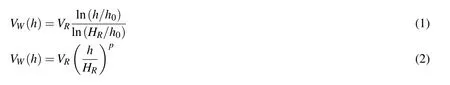
As the computational algorithms developed rapidly,there has been considerable research into offline optimization of DS trajectories,which offer more accurate numerical solution of minimum wind conditions required for DS.Sachs and Casta(2006)have set the fundamental problem of determining the minimum linear gradient required for DS with a high-performance sailplane.Based on the optimal trajectories for minimum wind gradient of a linear wind shear,[Bencatel,Kabamba,and Girard(2014)]derive a general equation of the necessary and sufficient conditions for sustainable DS with arbitrary aircraft models.However,the linear gradient model is only suitable to describe the wind gradient in altitude region rather than near the surface above which the horizontal wind speed varies irregularly with the altitude[Gao,Hou,Guo,Fan,and Chen(2014)].Zhao(2004)presents in-depth analysis into the optimal patterns and the least required wind gradient slop of glider DS using a direct collocation approach;the nonlinear correction coeff icient,A,is introduced into the linear wind model to represent the gradient variation with the altitude.However,the exponential-like wind profile(0＜A＜1)is not realistic as far as the authors know.Sachs(2005a)analyzes the minimum reference wind speed required for DS of albatrosses in a logarithmic wind field as shown by Eq.1.[Deittert,Richards,Toomer,and Pipe(2009a)]extend the work of Sachs by investigating trajectories for maximal wind conditions that allow DS and for max-imal cross-country travel rates along various directions.The optimization problem has be simplified by differential flatness and then implemented in AMPL software[Fourer,Gay,and Kernighan(2002)]and solved with the nonlinear solver IPOPT[W?chter and Biegler(2006)].Instead of the logarithmic wind model used by Sachs(2005a);Deittert,Richards,Toomer,and Pipe(2009a)use a popular power law model in wind energy engineering as shown by Eq.2.

Although there is no evidence that one of these two wind models is better or more realistic to describe the wind gradient profile than the other,they both involve three parameters used to denote reference wind strength(VR)at the reference height(HR)and to take into account the surface properties(h0,p),like irregularity,roughness and drag[Bencatel,Kabamba,and Girard(2014);Bencatel,Sousa,and Girard(2013);Farrugia(2003);Gualtieri and Secci(2011)].Sachs(2005a);Deittert,Richards,Toomer,and Pipe(2009a)only consider the minimum or maximum reference wind strength at a constant reference height and constant h0or p for DS.Lissaman(2005)discusses the optimal DS trajectories exploiting wind fields with various VRand HRat p=0.2.The 1/7 Power Law(p=0.1429)adopted by Deittert,Richards,Toomer and Pipe(2009a)has been used to describes atmospheric wind profiles over the surface sufficiently well during adiabatic conditions[Farrugia(2003)].Nevertheless,research has shown that power law exponent p is usually larger than 1/7.Moreover,the value of p depends upon the observed site and time on the order of hour,days and months[Farrugia(2003);Gualtieri and Secci(2011)].However,the analysis of the effect of various p on optimal DS trajectories is still lacking.Furthermore,in this paper,another limitation of the small p value is disclosed by introducing the constraint of strictly positive wingtip clearance[Deittert,Richards,Toomer,and Pipe(2009a)]in the trajectory optimization with a glider model.The more general feasible wind conditions which involve the minimum and maximum power law exponent and the minimal and maximal reference wind strength at different p are analyzed.

The engine assisted flight[Akhtar,Whidborne,and Cooke(2012);Sachs(2005b);Zhao and Qi(2004)]is the probable method to implement repeatable DS cycle in cases where the wind condition is out of the permissible domain for engineless flight.Other researchers turn to wind turbines and solar panels to extract more energy from other environmental sources during DS for on-board energy supplement[Bower(2011);Grenestedt and Spletzer(2010);Grenestedt and Spletzer(2010)].

However,these facilities are out of the scope of this paper.

Since the real-time wind field estimation method[Langelaan,Spletzer,Montella,and Grenestedt(2012)]and the trajectory tracking strategy for both powered[Akhtar,Whidborne,and Cooke(2012)]and unpowered[Bird,Langelaan,Montella,Spletzer,and Grenestedt(2014)]DS with small UAVs are more and more mature,this paper only focuses on the basic problem of designing the optimal DS trajectories for permissible wind conditions.Besides,the trajectory optimization often suffers from computational complexity.Akhtar,Whidborne,and Cooke(2012)showed that their optimization typically takes about 8 seconds to converge to a feasible solution on a standard desktop PC.Compared to the typical time for completing a DS cycle(9.6–10.9 s),the results is barely satisfactory for small UAVs with limited computational resources on-board.In effect,[Bird,Langelaan,Montella,Spletzer,and Grenestedt(2014)]trade computational complexity for on-board storage as they select the appropriate optimal path in real-time from the pre-computed ones across the range of expected aircraft speeds and wind conditions.In this paper,an efficient direct collection approach based on the Runge-Kutta integrator is used to solve the optimal trajectory in the AMPL[Fourer,Gay,and Kernighan(2002)]combined with IPOPT[W?chter and Biegler(2006)].The computational time is compared with the one in the work of Deittert,Richards,Toomer,and Pipe(2009a)due to use of the same software and solver.

2 Methodology

2.1 Wind field model

In this paper,the power law wind model given by Eq.2 is applied.The reference height can be picked arbitrarily and the authors follow Deittert’s choice of HR=20 m.The power law exponent p determines the distribution of the wind gradients along the altitude away from the surface.In general,lowest p values about 0.1 occur over smooth,hard ground,lake,or ocean,0.24 in areas with many trees or 0.3 in small towns,whereas higher values about 0.4 are found in urban areas with tall buildings[Gualtieri and Secci(2011)],and in the extreme case,values of 0.5–1.0 may be found for selected heights[Farrugia(2003)].Thus Deittert’s choice of p=0.1429 by which wind profiles over open oceans are matched well is no longer suitable for other surfaces with different roughness.Moreover,the p value varies with time and date at the same place.Therefore,it is worth studying on the optimal trajectories at different p values for small UAVs that are expected to accomplish persistent flight missions at any time and any place.The wind fields with different p values at VR=10 m/s are show in Fig.1(a).The reference wind speed VRrepresents the overall gradient and average speed of the wind profile that is shown in Fig.1b.

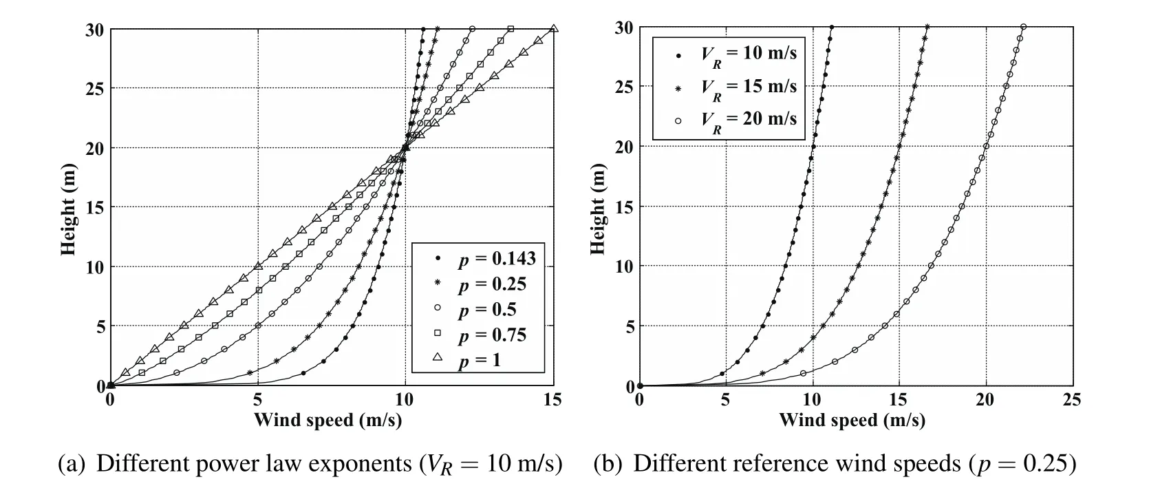
Figure 1:Wind fields with different parameters.

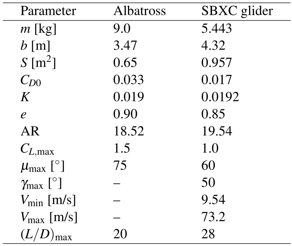
Table 1:Parameters for the flight models.

2.2 Flight model

There are two different flyers considered in this paper:an albatross and the SBXC glider.Their parameters are both listed in Tab.1.The albatross flight model and the numerical results given by Sachs and Bussotti(2005)are treated as benchmarks to validate the subsequent trajectory optimization method in this paper.While,the SBXC glider[Lawrance(2011)]is the main research object based on which the permissible wind conditions for optimal DS trajectories are discussed.The corresponding parameters of both models have the same order of magnitude and the values are very close.Particularly,the SBXC glider have higher maximum lift-todrag ratio,which indicates the potential of high performance of DS with the small UAV[Sachs and Casta(2006)].Besides,the maximum lift coefficient CL,max=1.0 and maximum bank angle μmax=60°of the SBXC glider are approximated by the SD2048 airfoil and the maximum load factor of 2.0 respectively[Lawrance(2011)].

The equations of motion(EOM)for a UAV given by Zhao(2004)in Eqs.3–8 is used in this paper:

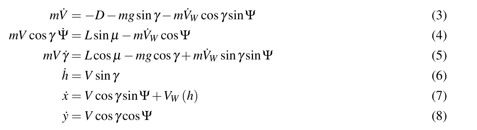
where L is lift force,D is drag force which are expressed as follows:

The drag coefficient CDdepends on the lift coefficient CL,yielding

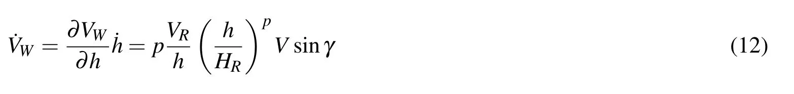
For the wind gradient is a quite steady phenomenon,the wind acceleration˙VWin the EOM only depends on the vertical wind gradient combined with the vertical speed of the vehicle itself:

The states of preceding EOM are airspeed V,heading angle Ψ,air-relative flight path angle γ,east,north positions x,y and the altitude h.The vehicle speed is modeled in a wind relative reference frame by Eqs.3–5 while the position is modeled in an earth fixed frame by Eqs.6–8.Actually,this EOM is simplified by omitting the side aerodynamic force,considering CLandμas control inputs directly and estimating drag force coefficient by Eq.11.Moreover,it does assume that a controller exists and is able to command and track a specified CLandμ.Under these assumptions,solving rotational motion equations and calculating moments are avoided subtly,thus the EOM has 3 DOF(degrees of freedom)and includes translational dynamics only.This simplified EOM is approximate enough and has been used for energy analysis and trajectory optimization in a significant amount of research about DS[Akhtar,Whidborne and,Cooke(2012);Bower(2011);Deittert,Richards,Toomer,and Pipe(2009a);Gao,Hou,Guo,Fan,and Chen(2014);Grenestedt and Spletzer(2010);Grenestedt and Spletzer(2010);Grenestedt,Montella,and Spletzer(2012);Lawrance(2011)].The advantage lies in the intuitiveness of using scalar airspeed V and flight path angle γ as state variables that are closely linked with effective energy of a UAV in the air-relative reference frame[Bower(2011)],while the speed and position in EOM adopted by Sachs(2005a);Sachs and Bussotti(2005)are both derived in the earth fixed frame.The primary disadvantage of these EOM appears when setting initial inertial speed that may be non-intuitive when the airspeed and the wind speed are very close for a trajectory problem[Bower(2011)].Although Zhao’s model[Zhao(2004)]is adopted in this paper due to preceding advantages,it should be emphasized that these two sets of EOM are equivalent.Thus,the optimal trajectory,which is obtained by Sachs’s model[Sachs and Bussotti(2005)]and used as the point of comparison,will satisfies Zhao’s model adopted in this paper.

2.3 Trajectory optimization using Runge-Kutta integrator

The flight model described by Eqs.3–8 can be treated as a nonlinear system:

wherex=[V,Ψ,γ,h,x,y]Tis the state vector,u=[μ,CL]Tis the control input vector.The optimal DS problem is to find an optimal controluto perform energyneutral flight subjecting to a certain objective and satisfying the nonlinear differential equations and some other terminal and path constraints.

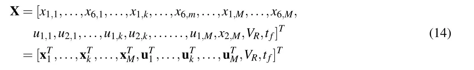
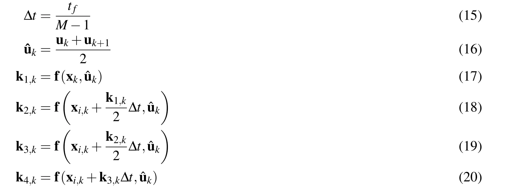
The optimal control problems for aircraft flight in time domain can be converted into pure parameter optimizations for numerical solutions[Hull(1997)].Deittert,Richards,Toomer,and Pipe(2009a)use differential flatness to achieve the conversion.A more efficient conversion method,the direct collocation approach,is used in this paper due to its flexibility,simplicity,and computational speed[Guo,Zhao,and Capozzi(2011)].In this approach,values of state and control variables are approximately represented as solution parameters at M discrete time nodes which are spaced equally within the solution time range[0,tf]:xi,kand uj,k,where k=1,2,...,M represents the kth node,i=1,2,...,6 represents the ith component of state vectorxand j=1,2 represents the jth component of control vectoru.Putting all the unknown parameters together,we have the design vector:

The explicit fourth-order Runge-Kutta integrator which has high accuracy in discretization[Hager(2000)]is used to approximate the nonlinear system Eq.13.For k=1,2,...,M?1,define:

Thus,the nonlinear system can be converted into 6(M?1)equality constrains as:

An ideal DS cycle is that the vehicle can come back to the initial states after flying across the wind field.The cycle is repeatable and energy neutral.Thus the terminal constraints for the free traveling DS pattern are:

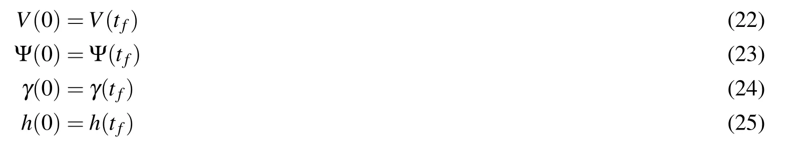
The free traveling pattern in which horizontal displacement of the vehicle is unrestricted is first defined as basic DS pattern by Zhao(2004)and also considered as the optimal DS pattern performed by the albatrosses[Sachs and Bussotti(2005)].If considering a strict closed loitering DS pattern,terminal position constraints defined by Eqs.26–27 should be added based on the free traveling pattern:

However,the heading angle constraint in Eq.23 only leads to eight-type trajectories.The more practical circular-type trajectories for stations keeping applications can be generated by setting 2π difference for terminal constraint on the heading angle as:

If a vehicle or an albatross is expected to gain net traveling speed toward a certain direction such as upwind,downwind or crosswind,the traveling DS pattern defined as cross-country DS pattern by Deittert,Richards,Toomer,and Pipe(2009a)can be studied by adding the following terminal constraints instead of Eqs.26–27:

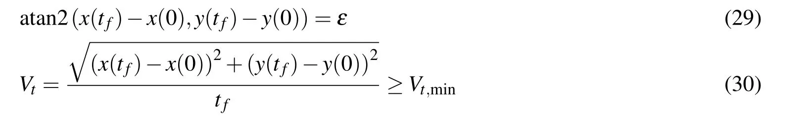
where ε is the traveling direction,Vtis the net traveling speed.The minimum travel speed Vt,minis used to prevent the resulting trajectories from becoming closed trajectories.

The initial conditions in all patterns are prescribed as:

In all the time nodes,the following path constraints should be satisfied:

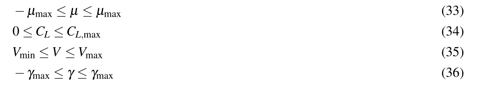
Particularly,the path constraint of strictly positive wingtip clearance[Deittert,Richards,Toomer,and Pipe(2009a)]is introduced to avoid collision between the vehicle and the surface:

The aim of this paper is to find the permissible wind conditions to support optimal DS of loitering and traveling patterns.According to the preceding wind model the wind conditions includes two factors:one is the power law exponent p;the other is reference wind strength VR.Thus,the main problem is to seek the minimum and maximum bounds of p andVRas follows:

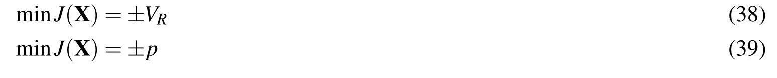
When using Eq.39 as the value function,the p is also treated as an unknown parameter and should be augmented in the design vector of Eq.14.

To sum up,the converted trajectory optimization problem can be stated to be finding a solution of the design vectorXthat minimizes the object value of Eq.38 or Eq.39,and satisfies the nonlinear differential constraints parameterized by Eq.21,the terminal constraints defined by Eqs.22–32 and the path constraints defined by Eqs.33–37.The optimization problem is implemented in AMPL[Fourer,Gay,and Kernighan(2002)],a modelling language for mathematical programming,and solved with IPOPT[W?chter and Biegler(2006)],a nonlinear mathematical programming solver.

2.4 Method validation

The solution methodologies from previous sections were validated by reproducing the numerical results for the problem of minimum wind strength of free traveling pattern DS given by Sachs and Bussotti(2005).Since the albatross has sophisticated flight technique in close proximity to the surface,the wingtip clearance constraint Eq.37 is not considered in the validation process.Instead,as in Sachs’s work,only a minimum height of the point mass above the surface is used:

Copying directly the figures from his work is not convenient for comparison,thus only the key parameters reflecting the characteristics of the trajectory are listed in Tab.2 such as minimum wind strength,cycle time,maximum height,travel direction and so on.

At first,the problem of minimum wind strength proposed by Sachs was solved using differential flatness(DF)method with the preceding software and solver[Deittert,Richards,Toomer,and Pipe(2009a)].The resulting trajectory is shown in Fig.2 by dash-dotted lines and airspeed and control inputs in Fig.3.These results and corresponding parameters in Tab.2 are almost identical with the results in Sachs’s publication[Sachs and Bussotti(2005)](see his Figs.6–10).The most significant difference is shown by a displacement difference along x axis of about 8m resulting in a minor numerical difference of less than 4°in travel direction.The difference is probably due to using different optimization methodology and software.Further,Deittert’s method was expounded very clearly in his paper[Deittert,Richards,Toomer,and Pipe(2009a)]and easy to implement.Thus,the results computed by their method were used as a more convenient and intuitive baseline for validating methodologies of this paper.In addition,comparing the computational times for different methods solving the same problem is more convincing due to use of the same software and solver.

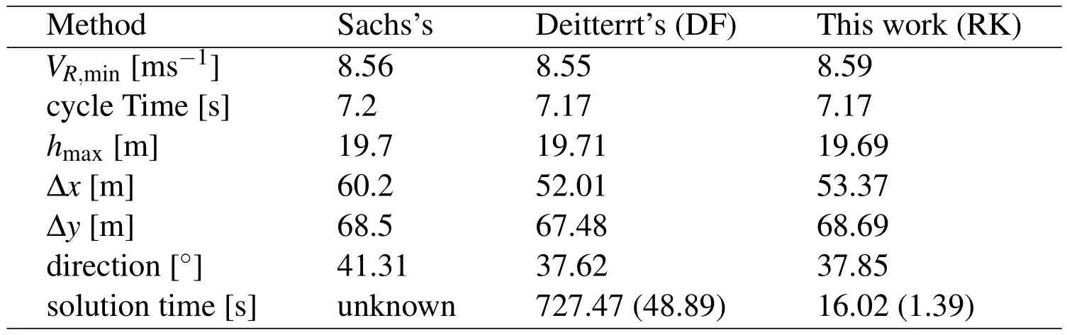
Table 2:Parameters of optimal trajectories with different methods.

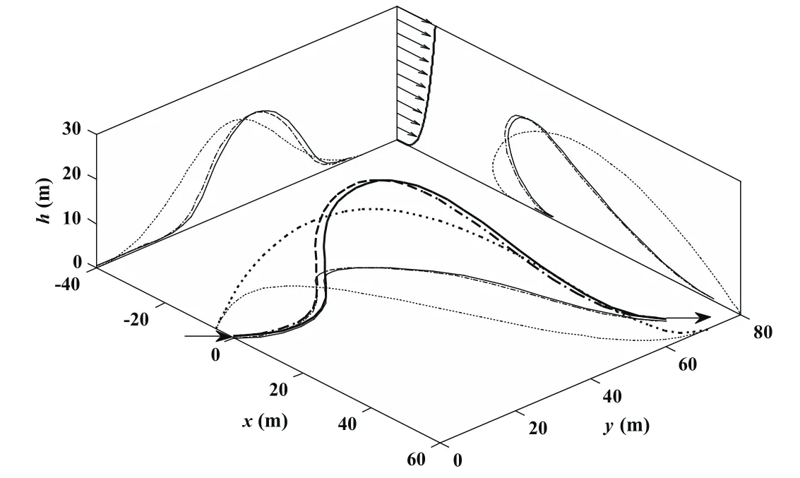
Figure 2:Albatross DS trajectory requiring minimum wind strength.

To be fair,all the optimization processes were implemented under Windows XP on the personal computer with Intel?Core?,i3-2100 CPU@3.10GHz.The number of time points of M=100 and the convergence tolerance of le-8 for all design variables,value function,and constraints were set for both methods.The number of frequency components N for the DF method was selected by empirical formula M=5N to achieve good results[Deittert,Richards,Toomer,and Pipe(2009a)].

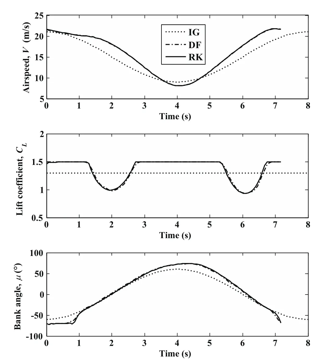
Figure 3:Albatross optimal DS trajectory parameters.

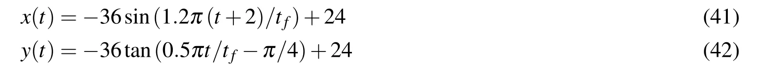
The initial conditions were first set to be 1.0 for all design variables and the solution time of about 12 minutes and 16s were obtained respectively.Although this setting of initial conditions for one method is not equivalent for the other one,it likely represents somewhat bad guesses for all design variables.The trajectory results marked by solid lines in Fig.2 and noted by“RK”short for Runge-Kutta in Fig.3 are identical with the ones of DF method.From the results of solution time in Tab.2,the RK method is more efficient than the DF method,however,the solution time of 16 s is still unsuitable for real-time applications.Thus,more proper initial conditions are expected to accelerate the convergence process.The curves of positions,states and inputs for the minimum wind trajectory in Sachs’s publication[Sachs and Bussotti(2005)]all have shape characteristics of trigonometric functions.Thus,the initial curves fitted manually by trigonometric functions according to his resulting figures were used for RK method.These initial guesses(IG,for short)are shown by Eqs.41–46 and by dotted lines in Figs.2–3.

The initial guesses of sinusoidal basis functions for DF method[Deittert,Richards,Toomer,and Pipe(2009a)]are converted from the ones of position time functions Eqs.41–43 by least-squares fitting method.The solution time plummets to 48.89 s and 1.39 s for DF and RK methods respectively under new initial guesses.

In sum,although both methods performs well in solving the optimal trajectory problem for DS,the RK method is far faster than the DF method under the proper initial conditions,making real-time implementation possible.The RK method will be used in the remaining sections of our work.

3 Limitation of the 1/7th wind power law for optimal dynamic soaring

The 1/7th Power Law(p=0.1429)has been used to describe the wind profiles over the surface in previous publications about DS[Deittert,Richards,Toomer,and Pipe(2009a);Sachs and Bussotti(2005)].However,when considering the minimum wind strength for the loitering DS pattern under terminal constraints of Eqs.22,24–28 and wingtip clearance constraint of Eq.37 where hmin=0 m for SBXC glider in the wind field of p=0.1429,the solver fails to give convergent optimizations.Similar situation can be found in free traveling pattern for both glider and albatross models.It indicates that the SBXC glider is unable to perform optimal DS under the wind field of p=0.1429 no matter how strong the reference wind VRis.

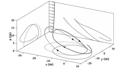
Figure 4:Closed trajectory for minimum wind strength and strictly positive height of point mass(dotted line)and the most proximal closed trajectory for strictly positive wingtip clearance(solid line)under the same wind condition:p=1/7,VR,min=3.88 m/s.

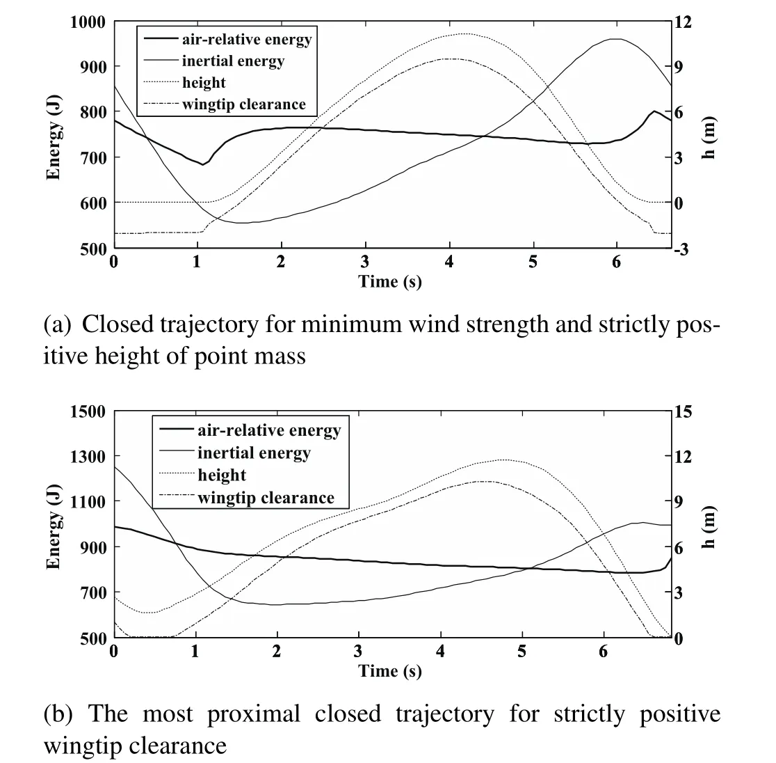
Figure 5:Air-relative energy,inertial energy,height and wingtip clearance for the trajectories in Fig.4.Wind condition:p=1/7,VR,min=3.88 m/s.

However,assuming that the wingtip clearance constraint of Eq.37 is loosened to the minimum height constraint of Eq.40 where hmin=0 m,the optimization process converges to a minimum VR=3.88 m/s for a closed circular trajectory as shown by dotted lines in Fig.4.Air-relative energy,inertial energy,height and wingtip clearance of this optimal trajectory are marked by thick solid,light solid,dotted and dash-dotted lines respectively in Fig.5(a).During this DS cycle,the UAV gains mechanical energy or ground speed through high altitude turn.It can be concluded by arbitrarily selecting two points at the same altitude in the upper curve of the height and analyzing the kinetic energy increase from the prior point before turning to the posterior point after turning.Further,the energy gain from the wind profile is proportional to the reference wind speed,VR[Sachs(2005a)].On the contrary,the UAV losses inertial energy during the low altitude turn and comes back to the initial state of inertial energy after finishing one DS cycle.Thus in the inertial fame,the trajectory can be characterized as the energy-neutral DS during which the energy gain from the wind profile is just sufficient to compensate for the energy loss due to drag.Figure 5(a)shows that the air-relative energy has a gently downward trend during the high altitude turn and decreases fast during the low altitude turn where the airspeed is larger as well as the energy loss due to drag.The air-relative energy gain mainly occurs at the moments of upwind climb and downwind dive at low altitude where the wind gradients are the largest in the whole wind profile of p=0.1429(see Fig.1(a)).It is because the air-relative energy gain depends linearly upon the wind gradient when the UAV climbs upwind or dives downwind according to the “dynamic soaring force”theory[Barnes(2015);Deittert,Richards,Toomer,and Pipe(2009a)].As seen from Fig.5(a),the UAV recovers the air-relative energy when coming back to the initial position after one DS cycle,which indicates a balance between the energy gain and the energy loss,and an energy-neutral DS cycle in the air-relative frame.To sum up,the DS process is the unification of the energy-neutral cycles both in the inertial frame and in the air-relativeframe.The energy gain of the former cycle originates from the reference wind speed VRat higher altitude,while the energy gain of the latter cycle from the wind gradients depending on the wind parameter p at lower altitude.However,the downward wingtip is about 2 m below the surface when the vehicle flies at low altitude.The albatrosses are perhaps unable to perform this trick,let alone the UAVs.

Reconsidering the positive wingtip clearance constraint of Eq.37 and removing the terminal position constraint of Eqs.25–27,the most proximal closed trajectory under the same wind condition(p=0.1429,VR=3.88 m/s)is computed in order to disclose the handicaps in performing circular trajectories.The optimal trajectory for the value function of minimum terminal position difference in Eq.47is noted by solid lines in the Fig.4 and the corresponding energy states are shown in Fig.5(b).

The variation of inertial energy is very similar to the one in the minimum wind strength trajectory as shown in Fig.5(a)However,while turning at low altitude,the vehicle(point mass)cannot approach the surface where large wind gradients exit because of keeping the strictly positive wingtip clearance.The air-relative energy therefor cannot achieve two typical increases during upwind climb and downwind dive as shown in Fig.5(a)and the energy extracted from the air mass cannot support a closed trajectory as well as an energy-neutral cycle.The terminal position difference only reflected in the height in Fig.4 indicates the energy shortfall.

In sum,the limitation of the wind field of p=0.1429 for DS is that the vertical range of wind gradients at low altitude is too narrow to be exploited by the UAV with a banked and long wingspan.As seen from Fig.5(a),the vertical distribution of wind gradients depends on the power law exponent p in a wind field.The vertical range of large gradient is extended with increasing p.Although the wind gradient over there is smaller under a larger p,the opportunity that the UAV can use the strong wind gradient will increase due to its higher location.Considering the analysis above,the reference wind speed VRis only one aspect of the permissible wind conditions for DS and the power law exponent p is another key factor affecting the energy-gain process.Additionally,the p value is influenced by many factors including time,season and site,so that the p value should be included when considering the permissible wind conditions for DS.

4 Permissible wind conditions for loitering dynamic soaring

4.1 Minimum and maximum feasible power law exponent

In this section,the feasible p values of the wind field for loitering DS patterns with the SBXC glider are investigated.Setting the same terminal constraints especially for closed and circular trajectories,considering the strictly positive wingtip clearance as the last section,and adding the parameter p into the design vector,the trajectory optimization problems for minimum and maximum feasible p values are solved.

The range of p values is determined using Eq.48 according to the real situations of wind fields in nature as described in Sec.2.1.

The terminal constraint for reference wind strength defined by Eq.49 is determined by the extreme wind speed observed in hurricanes[Schott,Landsea,Hafele,Lorens,Taylor,Thurm,Ward,Willis,and Zaleski(2012)].

The trajectory optimization for minimum p converges to 0.2146 selecting the reference wind strength of VR=12.0032 m/s.The closed trajectory and trajectory parameters for the minimum power law exponent is noted by dark-gray lines in Figs.6–7.When solving the most proximal closed trajectory at the wind field with p=0.1429 and the same reference wind strength of VR=12.0032 m/s,the resulting trajectory and the energy variation are very similar to the case of VR=3.88 m/s in Figs.4 and 5(b)although the reference wind speed here is much stronger than that in those figures.The terminal position difference shown only in the height indicates the vehicle cannot execute energy-neutral DS in the air-relative frame due to the narrow vertical range of strong wind gradient at low altitude when p=1/7.The minimum feasible p value is slightly larger than 1/7.As the range of low altitude wind gradient increases with the increasing p value,there is more effective energy gained by the UAV during upwind climbing and downwind diving at low altitude.When the p value reaches the minimum feasible value,the vehicle just obtain enough energy from the wind field to perform strictly closed trajectory as well as the energy-neutral cycle.

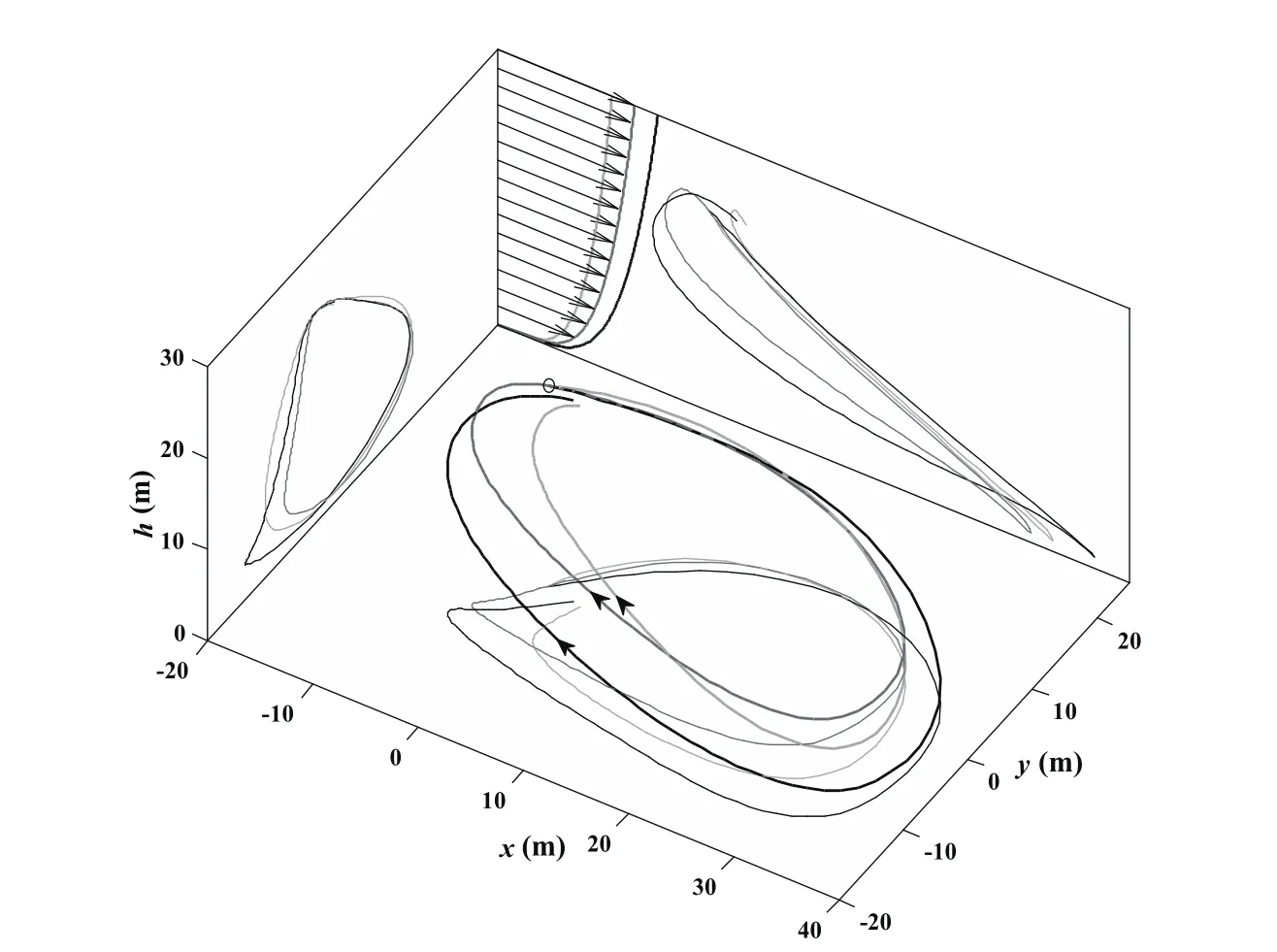
Figure 6:Closed trajectory for minimum p selecting VR=12.0032 m/s(dark gray lines)and the most proximal closed trajectories for VR=10 m/s(light gray lines)andVR=14 m/s(black lines)at the wind field with the minimum p.

More interestingly,with the fixed value of p=0.2146,solving the optimization problems for minimum and maximum reference wind speed respectively according to Eq.38,the resulting objective function values are very close toVR=12.0032 m/s which is selected by the optimization process for minimum p,and the deviations are within 10?5.This indicates that the reference wind speed of VR=12.0032 m/s is the unique permissible wind condition for the wind field with p=0.2146.

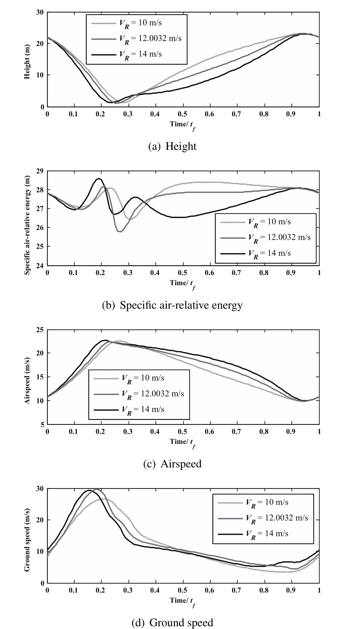
Figure 7:Trajectory parameters for optimal DS cycles in Fig.6.

In order to explain why other values of VRdo not support closed trajectory DS,take the most proximal closed trajectories for VR=10 m/s and VR=14 m/s in the wind field with the minimum p for example.For sake of comparison,these two trajectories and their parameters are superposed in Figs.6 and Fig.7 by light-gray lines and black lines respectively.There is no height(potential energy)difference between the start and end points for both situations and the terminal constraint of airspeed defined by Eq.22is also satisfied,thus the energy-neutral cycles havebeen realized for both air-relative and inertial frames.However,the terminal position differences are mainly presented in the downwind direction(positive x coordinates).In the first place,the overall wind gradients in the wind field with VR=10 m/s decreases compared to the feasible wind field for minimum p.As can be seen form Fig.7(b),compared to the height shown in Fig.7(a),the UAV not only utilizes the limited wind gradients at low altitude but also be willing to use the wind gradients at higher altitude during the upwind climb to gain energy.As Fig.7(a)shows,the UAV promptly climbs after low altitude turn and the potential energy increases,while the air-relative kinetic energy decreases(see Fig.7(c)).Although the air-relative total energy is also increasing as shown in Fig.7(b),the available overall energy contained in the wind field with weaker VR,after all,is limited.Thus,the airspeed(air-relative kinetic energy)is smaller than that of the trajectory for minimum p as shown in Fig.7(c).Besides,the headwind is relative stronger at higher altitude so the ground speed along the upwind direction is weaker(see Fig.7(d)),and then,the displacement in the direction of negative x coordinates during upwind climb decreases obviously(see Fig.6).Finally,the UAV cannot come back to the start place after high altitude turn due to the drift.

On the contrary,the overall wind gradients in the wind field with VR=14 m/s are larger than that in the feasible wind field for minimum p as well as the overall wind speed.To avoid the strong wind at higher altitude,the UAV tends to fly upwind at somewhat lower altitude,as shown in Fig.7(a).To compensate the drift during upwind climb,the UAV is forced to fly faster relative to the wind compared to the minimum-p trajectory(see Fig.7(c)).

However,the UAV must perform the high altitude turn from upwind direction to downwind direction to close the trajectory and come back to the initial airspeed to achieve the energy-neutral.As Fig.7(c)shows,the airspeed for trajectory of VR=14 m/s decreases to almost the same as the minimum-p trajectory during the high altitude turn.Due to the larger wind speed at high altitude in the wind field with VR=14 m/s,the downwind drift increases as well as the displacement in the direction of positive x(see Fig.6).Therefore,the UAV misses the initial point after the high altitude turn.Although the UAV beforehand struggled against the headwind by using the energy gained from the wind gradient while climbing(see Fig.7b)to get more displacement in the upwind direction than that in minimum-p situation(see Fig.6),the high altitude drift is still too strong to be compensated.The trajectory optimization for maximum power law exponent always converges to the up boundary of p value domain,p=1.0.However,the selected reference wind speeds are different when using different initial guesses to solve the same optimization problem.In other words,in the wind field with p=1.0,the reference wind speed supporting the closed trajectory DS is not unique.

4.2 Permissible wind condition boundary

From the analysis in last subsection,it can be predicted that the feasible range of VRfor closed DS increases from the sole point to a wide domain as the p value increases.In this subsection,the minimum and maximum VRfor each feasible p value are computed by the trajectory optimization using Eq.38 as the cost function.It is run for pvalue range from0.25to1.0in steps of0.05increments and the results in combined with the minimum p point are shown in Fig.8.The maximum VRvalue increases rapidly while the minimum VRvalue gradually decreases with increasing p value.Particularly at the p value slightly larger than the minimum,the feasible VRrange extends significantly due to the soaring maximum feasible VR.When p value is larger than 0.625,the theoretical value for maximum VRexceeds the up limit of the constraint for VRin Eq.49.Thus,the maximum VRis restricted to the value equal to 70 m/s according to the natural truth in the optimization process.

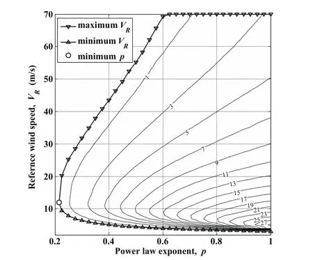
Figure 8:Permissible wind conditions for loitering DS with SBXC glider.

As the p value increases,the vertical range of the large wind gradient in the wind field is extended,and in the meantime,the high altitude wind gradient increases,as illustrated in Fig.1(a).Thus,the UAV can gain almost equivalent energy for closed trajectory DS even in a wind field with a smaller VRwhich determines the overall gradient of the wind pro file.On the other hand,more energy can be obtained by the UAV in the wind field with higher p and higher VR,to conquer the strong headwind at high altitude.Besides,the overall wind speed is reduced with increasing p value(see Fig.1(a)),thus the drift while climbing has a deceasing trend which is favorable for closing the DS trajectory loop.The UAV therefor can get more displacement during the upwind climb phase at relative lower altitude preparing the high altitude turn even ifthe VRis higher.

The curves of maximum and minimum VRfor different p values constitute the boundary of a bell-shaped domain for permissible wind conditions.The point of minimum p value is the top of the “bell”and the line segment joining the points of maximum and minimum VRfor p=1.0 forms the bottom of the “bell”.As long as the combination of VRand p values falls inside the bell-shaped domain,it can be considered as a permissible wind condition for closed trajectory DS.

4.3 Permissible wind conditions for maximizing the minimum allowable wingtip clearance

The preceding permissible wind conditions are based on the critical wingtip clearance constraint of Eq.37 where hmin=0 m,which indicates the vehicle wingtip might just touch the surface during DS,especially at the stage of the low altitude turn.It is a challenge for the guidance and control to follow the optimal DS trajectory with a long wingspan vehicle,particularly,the turbulence always exists in the wind field near the surface[Deittert,Richards,Toomer,and Pipe(2009b)].Besides,there are measurement errors in avionics(for example,the altimetric sensor),thus the scrapes and collisions between the wingtip and the surface seems inevitable.Furthermore,the increasing p value implies the increasing height of humps or obstacles on the surface as described in Sec.2.A.It is obvious that increasing the clearance between the wingtip and the surface can make the whole system more robust,safe and applicable while performing stationary DS in different circumstances.

Selecting each point of p and VRvalues in the bell-shaped domain as the known conditions,the closed trajectories for maximizing the minimum wingtip clearance defined by Eq.50 can be computed.

Running the trajectory optimizations for p value varying from 0.25 to 1.0 at 0.05 step interval and integral VRvalues between the minimum and the maximum for each p value,the results for the maximum lower bound of wingtip clearance(hmin)are obtained and marked by the contour plot in Fig.8.The unit of the maximum hminvalue marked in each contour is meter.For each p value,the maximum values of hminat the maximum and minimum VRare both almost zero and the corresponding trajectories are identical with the trajectories for the maximum and minimum VRusing the constraint of strict positive wingtip clearance except the situations that VRis forced to equal 70 m/s.It can be inferred that the positive wingtip clearances is a crucial constraint for feasible VRrange.The maximum hminincreases at first and reduces afterwards with increasing VR.It is because the larger wind gradient in the wind field,particularly in higher altitude,reduces the dependence for gaining energy on the strong wind gradient at low altitude;in the meantime,the increasing overall wind strength speeds up the drift the vehicle tend to maneuver at lower altitude in turn.

When the p value is relatively large,the wind field can be treated almost as linear wind profile and the VRlinearly determines the wind gradient slope as shown in Fig.1(a).Thus the maximum and minimum VRvalues at p=1.0 represent the critical constant wind gradient for closed DS trajectories.As the VRincreases slightly from the minimum VRvalue for large p values,the overall wind gradient increases rapidly and the wind strength is still weak.The maximum hminshows a dramatically upward trend because there is consistent wind gradient in the whole wind profile and the small drift at higher altitude has little effect on the DS process.

For the same VRat the permissible domain,the maximum hminbecomes larger with increasing p value.On the one hand,there is larger wind gradient available for energy extraction at high altitude with larger p value for the same VR.On the other hand,the high altitude wind blows more weakly as p value increases and,hence the driftdecreases.Moreover,the VRat the extreme value for the maximum hminat each p gradually decreases from about 12 m/s to 5 m/s as p value increases.It indicates that the increased wind gradient at high altitude depending on increasing p value exceeds the reduction due to decreasing VRvalue in terms of energy extraction by the DS vehicle.Besides,the slightly smaller VRvalue reduces the overall wind speed as well as the drift.

To sum up,if the guidance and control system has a maximum error of 2 m in height for DS trajectory tracking under persistent turbulence and the height of obstacles on the surface are within 3 m,the permissible wind conditions become a shrunk bell-shaped domain which boundary is determined by the maximum hmincontour of 5 m.

4.4 Sensitivities of the permissible wind conditions to vehicle model parameters

Section 3 has shown that the long wingspan of the vehicle restricts the utilization of large wind gradient at low altitude and it can be concluded from Sec.4.3 that the wingtip clearance is a key factor to determine the permissible domain of wind conditions for close DS.It implies that reducing the wingspan can improve the performance of extracting energy from wind field in terms of the range of the permissible domain for wind conditions.Thus,the effect of changing wingspan on the permissible domain under the same constraint of minimum wingtip clearance is considered significantly in this section.

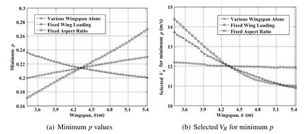
Figure 9:Variation of minimum p point with changing wingspan.

At first,considering the permissible domain based on the model parameters for the SBXC glider as the baseline case,the sensitivity of the minimum power law exponent to the wingspan b is investigated by repeatedly solving the optimization problem while changing the b value alone between runs and the results are shown by circles in Fig.9(a).The corresponding VRvalues at the points for minimum p are shown in Fig.9(b).Then,the permissible wind condition boundaries for two typical wingspan values around the baseline case(b=3.42 m and b=5.22 m)are computed and shown in Fig.10(a)to illustrate the changing of the whole permissible domain with the variation of wingspan.As Fig.9 shows,the minimum p value decreases slightly with shorter wingspan,while the VRvalue remains around 12m/s.Figure 10(a)illustrates that the minimum p point moves to the left and the permissible domain is expanded as the wingspan decreases.The permissible boundary curve of the baseline case which is actually between the example curves is omitted hear to avoid unclearness.This can be thought of as a validation for the implication at the beginning of this section.In fact,to change the wingspan alone is equivalent to loosening the constraint of minimum wingtip clearance.Thus,the vehicle center of gravity can reach the lower altitude with stronger wind gradient and the range of allowable reference wind speed extends at each p value.

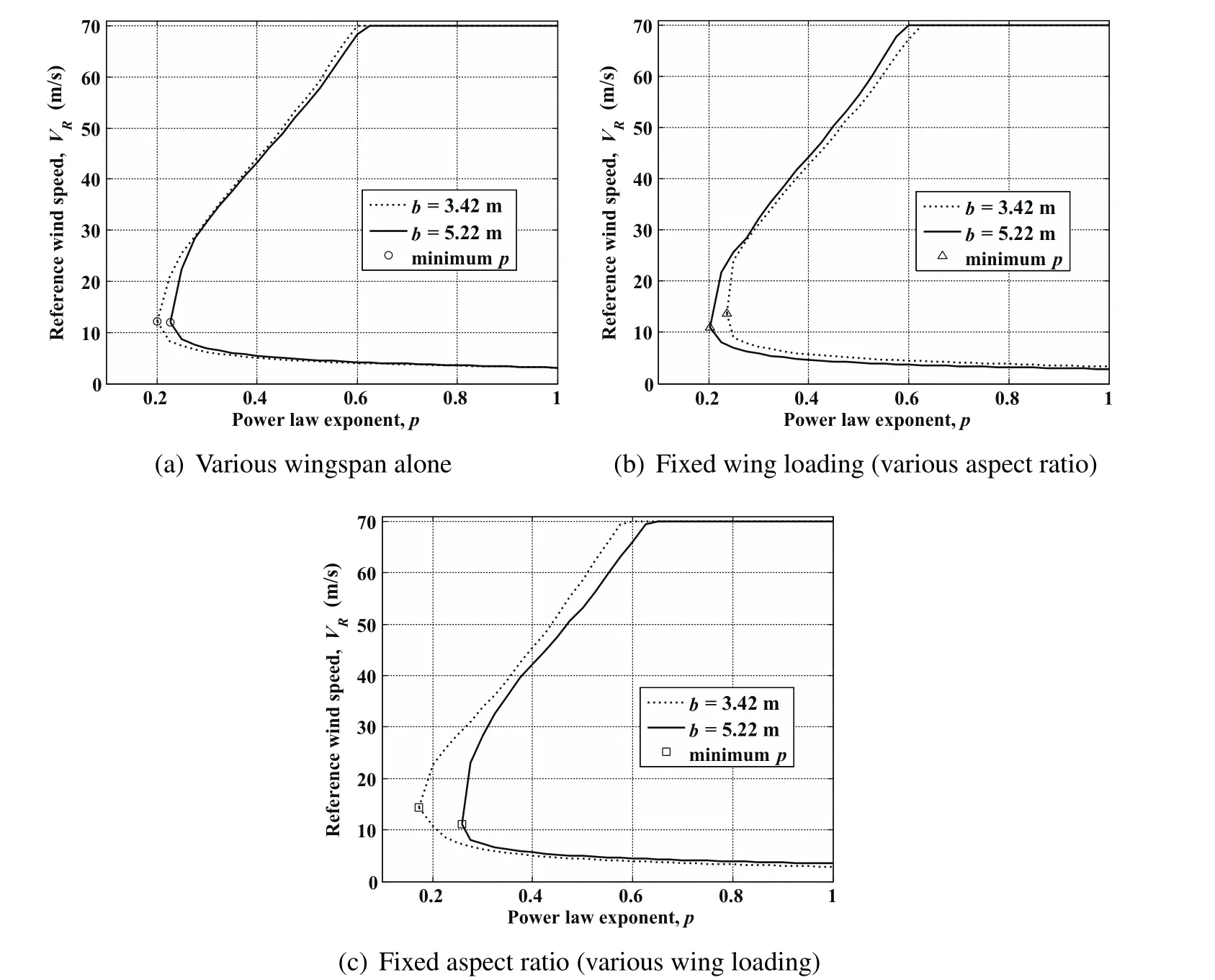
Figure 10:Permissible wind condition boundaries for b=3.42 m and b=5.22 m respectively.

However,the extension of permissible domain with deceasing wingspan is not very obvious.In the past,two more important parameters affecting the required wind conditions for DS have been discussed:the maximum lift-to-drag ratio,(L/D)max,and the wing loading,m/S[Sachs and Casta(2006);Sukumar and Selig(2013)],which are also key parameters of flight performance in conceptual design of aircraft[Raymer(1992)].The changing wingspan just has impacts on these two parameters.According to Eq.11 the maximum lift-to-drag ratio is

Decreasing the wingspan alone reduces the aspect ratio(AR)which is defined as the ratio of the wingspan to the average wing chord and results in smaller(L/D)max.In the meantime,it reduces the wing area and then increases the wing loading.These impacts are not considered in above discussion about changing the wingspan alone.

In order to decouple the impacts due to those two parameters,the wing loading is set to be fixed at first in the following discussion.When the wingspan becomes shorter,the wing chord is extended to keep a constant wing area.The(L/D)maxbecomes smaller due to decreasing AR.In this case,the minimum p points and the corresponding VRvalues for AR ranging from 12.22 to 30.70 are shown by triangles in Fig.9 and the permissible domains for b=3.42 m and b=5.22 m are shown in Fig.10(b).The minimum p point moves toward upper right on the p-VRplane with decreasing wingspan.Although the variation of VRbecomes greater,these two boundary curves do not form strict intersections.The permissible domain is shrunk inward with the deceasing wingspan under the same wing loading instead of be expanded when reducing the wingspan alone.Thus,the size of permissible domain shows an increasing trend as AR increases because larger(L/D)maxmeans smaller drag force and consequently less energy required extracting from wind field.It also implies that the effect of increasing AR and remaining constant wing loading while increasing the wingspan to expand the permissible domain exceeds the effect to reduce due to only extending the wingspan.

Then,considering the fixed AR,the wing loading increases from 3.62 kg/m2to 9.09 kg/m2as the wingspan becomes shorter and consequently the wing area decreases.In such case,the p value noted by rectangles in Fig.9(a)decreases more signif icantly than the situation of only decreasing the wingspan.Figure 10(c)shows that the minimum p point moves to upper left and the permissible domain boundary extends outward with decreasing wingspan.

Furthermore,since the wingspan can influence the permissible domain of wind conditions for closed DS through directly changing(L/D)maxand m/S,the parasitic drag coefficient CD0which is another parameter affecting(L/D)maxaccording to Eq.51 and the vehicle mass m which also determines the wing loading obviously should be considered in the sensitivity analysis.Figure 11 shows that the minimum p value is reduced linearly with decreasing CD0because of the direct effect of improving(L/D)maxand the selected VRvalue remains stable at around 12 m/s.It can be inferred that the permissible domain of wind conditions would be enlarged outward as CD0decreases.

Moreover,as Fig.12 shows,the minimum p value sees a downward trend with increasing m due to the larger wing loading.It also implies that the size of permissible domain would be expanded with increasing m.High vehicle mass is beneficial to perform closed DS even in the wind field with small p value in which the practicable wind gradient is limited because the “dynamic soaring force”defined in[Barnes(2015);Deittert,Richards,Toomer,and Pipe(2009a)]depends linearly on the UAV’s mass.It also can be noted that the decreasing of p value become gentle with increasing m because the larger wing loading usually results in higher average lift coefficients and larger airspeed[Deittert,Richards,Toomer,and Pipe(2009a)]which cause more energy loss due to drag[Eqs.10–11].

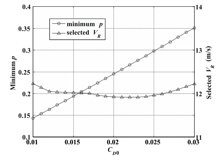
Figure 11:Variation of minimum p point with changing parasitic drag coefficient CD0.

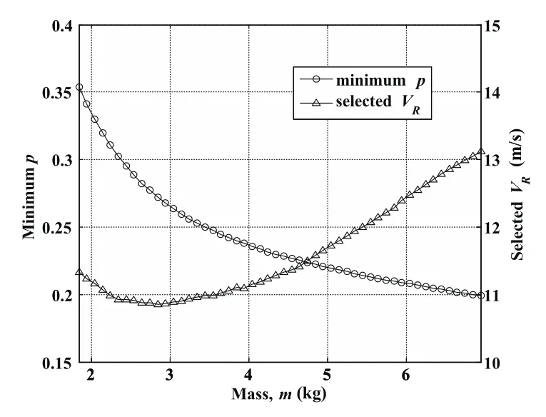
Figure 12:Variation of minimum p point with changing vehicle mass m.

To sum up,the point of minimum p value is used to moving on the p-VRplane with changing vehicle parameters.It reflects the variation of the permissible domain of wind conditions for close DS to some extent.To reduce the wingspan alone cannot obviously improve the efficiency of gaining energy from gradient wind fields;however,if properly increasing the maximum lift-to-drag ratio and the wing loading,the point of minimum p value will move toward the left on the p-VRplane and the permissible domain will be enlarged.

5 Permissible wind conditions for traveling dynamics soaring

5.1 Permissible wind conditions for upwind dynamic soaring considering the maximum traveling speed

The other possible applications of periodic DS are getting net inertial speed toward different directions in the reconnaissance and survey missions over open areas.Take the upwind DS that is the extreme and hardest situation[Richardson(2015)]for example,the permissible wind conditions for traveling DS are analyzed.To compute the upwind traveling DS trajectories,the constraints of Eqs.29–30 where ε=90°and Vt,min=0.5 m/s are required to ensure displacement along the expected traveling direction.The constraint of wingtip clearance is also considered and for comparison’s sake,hmin=0.25 m is selected in all the optimization processes.The result for minimum power law exponent is p=0.2069 selecting VR=12.8617 m/s and the net traveling speed is just the minimum,Vt=0.5 m/s.Like the closed trajectories,the maximum and minimum VRat minimum p are identical with the VRvalue selected by the optimization for minimum p.The maximum power law exponent is always 1.0 and the selected VRvalues are various when using different initial guesses.The curves of maximum and minimum VRversus p form a bellshaped domain in Fig.13,which illustrates the permissible wind conditions for upwind traveling DS.

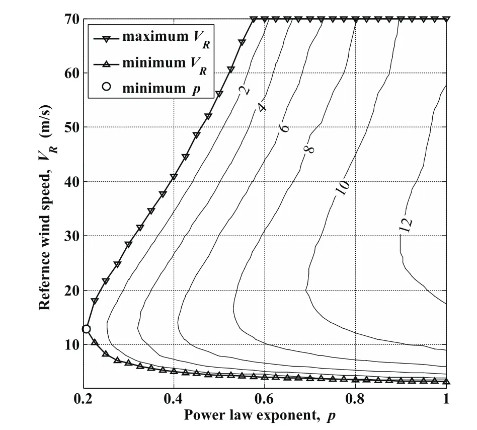
Figure 13:Permissible wind conditions for upwind traveling DS with SBXC glider.

The UAV is usually expected to fly from one point to another point as fast as possible,thus the trajectory optimization for maximum traveling speed described by the value function in Eq.52 is considered.

where Vtis defined by Eq.30.Running the trajectory optimization at each point within the bell-shaped domain,the results of maximum Vtare obtained and shown by the contour plot in Fig.13.The unit of the velocity value marked in each contour is m/s.Like the boundary of permissible domain for loitering DS trajectories,the lines of maximum and minimum VRare identical with the contour of Vt,max=0.5 m/s for upwind traveling DS trajectories except the situation of 70 m/s.It implies that the constraint of minimum Vtin Eq.30 determines the feasible VRrange.

For the same p value,the maximum Vtincreases at the beginning and drops latter as the reference wind becomes stronger.The increasing VRmeans more wind gradient energy that can be extracted from the wind field by the UAV to support the upwind traveling.However,the increasing VRalso causes more downwind drift and in order to keep the inertial speed,the UAV requires larger airspeed but loses more energy due to drag.For the same VR,the maximum Vtincreases with the p value because the increasing p value enhances not only the opportunity of using the large gradient at low altitude but also the wind gradient at higher altitude.Additionally,the smaller wind speed below the reference height due to the larger p value is favorable for upwind traveling.

In sum,if the mission requirement for the UAV is to travel upwind with an average inertial speed larger than 6 m/s for example,the permissible wind conditions becomes a shrunk bell-shaped domain which boundary is determined by the contour of Vt,max=6 m/s.

5.2 Permissible wind conditions for different traveling directions

Using the same method for calculating the permissible domain of upwind DS,the permissible wind conditions for different traveling directions can be computed by setting various traveling direction ε and repeatedly solving the optimization problem.As ε increases from ?90°to 90°,the minimum p value allowing traveling DS shows a decreases trend as shown in Fig.14(a).The permissible domain boundaries consisting of minimum and maximum VRcurves for representative traveling directions of ε=90°,?45°,0°,45°and 90°are shown in Fig.15.According to the sensitivities of the permissible domain to model parameters,the displacement of minimum p point on the p-VRplane determines the size of the whole permissible domain.Similarly,the permissible domain expands due to that minimum p point move toward left on the p-VRplane with increasing ε as shown in Fig.15.

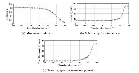
Figure 14:Variation of minimum p point with changing traveling direction ε.

Figure 15:Permissible wind condition boundaries for different traveling directions ε.

When ε＜ 0°,the minimum p value decreases within a small range compared with the one for ε=90°(upwind).Although the VRvalue increases slightly(see Fig.14(b)),the boundaries of permissible domains for ε＜ 0°are basically coincident.Just in the time of the traveling direction changes from upwind to downwind(ε=0°),the p value and VRvalue begin to change rapidly with increasing ε.As a result,the permissible domain for traveling DS is expanded,especially the area for relative smaller p and larger VRas shown in Fig.15.When ε＞ 75°,the p value decreases to the value below 0.05 and the selected VRvalue reaches the allowable maximum.It means that the vehicle would mainly use the wide range wind gradient determined by VRrather than the narrow layer of larger wind gradient.Since the downwind traveling DS cases have larger permissible domain of wind conditions than the upwind situation,they are said here to be more efficient.It is because the vehicle performing upwind traveling DS has to overcome the drift,while in the downwind situation,the vehicle can utilize the drift to obtain traveling speed toward specific directions.

It also can be noted that the traveling speed at minimum p point is always 0.5 m/s which limited by Eq.30 when ε＜ 0°,increases rapidly when ε＞ 0°and reaches about 67 m/s which is even close to the maximum allowable VRwhen ε＞75°.It implies that,the vehicle benefits from the drift to get lager traveling speed under the same wind conditions within the permissible domain during downwind traveling DS than the upwind traveling situation.

6 Conclusions

This paper shows the general feasible wind conditions that involve the power law exponents(p)and the reference wind strengths(VR)at different p values for loitering and traveling patterns of optimal DS.To solve the optimal DS trajectories,an efficient direct collection approach based on the Runge-Kutta integrator is used.The little computational time of this method indicates potential real-time applications for the CPU on-board a small UAV.

The wind field with p=1/7 cannot support DS with SBXC glider because the vertical range of larger wind gradients at low altitude which is determined by p value is too narrow to be exploited by the UAV with a banked and long wingspan.Moreover,the p value usually does not accord with the 1/7th Power Law and also depends upon the observed site,the time and the date.Thus,this paper emphasizes the effect of p value on the permissible wind conditions for DS.

For the loitering DS,the optimization results for minimum and maximum VRat different p values show that the maximum VRincreases rapidly while the minimum VRgradually decreases with increasing p value within the allowable range.The feasible range of VR,which increases from the unique point of permissible wind condition(p=0.2146 and VR=12.0032 m/s)to a wide domain at p=1.0,forms a bell-shaped domain for permissible wind conditions.The permissible domain is shrunk with increasing maximum smallest allowable wingtip clearance trading for robustness and safety of the vehicle system.Sensitivities of the permissible domain to vehicle model parameters show that loitering DS is more efficient in terms of the permissible domain size when properly reducing the wingspan and increasing the maximum lift-to-drag ratio and the wing loading of the soaring-capable vehicle.

For the traveling DS,similar bell-shaped domain of permissible wind conditions can be found.The permissible domain is shrunk when improving the requirement for traveling speed.When the traveling direction changes from upwind to downwind,the permissible domain for traveling DS is expanded,especially the area for relative smaller p and larger VR.The downwind traveling DS benefits from the wide range wind gradient and the drift due to VRinstead of the narrow layer of larger wind gradient determined by p value.

Akhtar,N.;Whidborne,J.F.;Cooke,A.K.(2012):Real-time optimal techniques for unmanned air vehicles fuel saving.Proceedings of the Institution of Mechanical Engineers,Part G:Journal of Aerospace Engineering,vol.226,pp.1315-1328.

Barnes,J.P.(2015):Aircraft energy gain from an atmosphere in motion:dynamic soaring and regen-electric flight compared.in AIAA Aviation:AIAA Atmospheric Flight Mechanics Conference,Dallas,TX,22-26 June,AIAA Paper 2015–2552.

Bencatel,R.;Kabamba,P.;Girard,A.(2014):Perpetual dynamic soaring in linear wind shear.Journal of Guidance,Control,and Dynamics,vol.37,no.5,pp.1712-1716.

Bencatel,R.;Sousa,T.J.D.;Girard,A.(2013):Atmospheric flow field models applicable for aircraft endurance extension.Progress in Aerospace Sciences,vol.61,pp.1–25.

Bird,J.J.;Langelaan,J.W.;Montella,C.;Spletzer,J.;Grenestedt,J.(2014):Closing the loop in dynamic soaring.in AIAA Guidance,Navigation and Control Conference,National Harbor,Maryland,13–17 January,AIAA Paper 2014–0263.

Bower,G.C.(2011):Boundary layer dynamic soaring for autonomous aircraft design and validation.Ph.D.Thesis,Stanford University.

Deittert,M.;Richards,A.;Toomer,C.A.;Pipe,A.(2009a):Engineless unmanned aerial vehicle propulsion by dynamic soaring.Journal of Guidance,Control,and Dynamics,vol.32,no.5,pp.1446–1457.

Deittert,M.;Richards,A.;Toomer,C.A.;Pipe,A.(2009b):Dynamic soaring flight in turbulence.in AIAA Guidance Navigation and Control Conference,Chicago Illinois,10–13 August,AIAA Paper 2009–6012.

Farrugia,R.N.(2003):The wind shear exponent in a mediterranean island climate.Renewable Energy,vol.28,pp.647–653.

Fourer,R.;Gay,D.M.;Kernighan,B.W.(2002):AMPL:a modeling language for mathematical programming(2nd ed.),Thomson,Duxbury,MA.

Gao,X.;Hou,Z.;Guo,Z.;Fan,R.;Chen,X.(2014):Analysis and design of guidance strategy for dynamic soaring with UAVs.Control Engineering Practice,vol.32,pp.218–226.

Grenestedt,J.L.;Spletzer,J.R.(2010):Optimal energy extraction during dynamic jet stream soaring.in AIAA Guidance,Navigation,and Control Conference,Toronto,Ontario Canada,2–5 August,AIAA Paper 2010–8036.

Grenestedt,J.L.;Spletzer,J.R.(2010):Towards perpetual flight of a gliding unmanned aerial vehicle in the jet stream.in 49th IEEE Conference on Decision and Control,Atlanta,GA,USA,December 15–17.

Grenestedt,J.;Montella,C.;Spletzer,J.(2012):Dynamic soaring in hurricanes.in International Conference on Unmanned Aircraft Systems,Philadelphia,US,12–15 June.

Gualtieri,G.;Secci,S.(2011):Wind shear coefficients,roughness length and energy yield over coastal locations in southern italy.Renewable Energy,vol.36,no.3,pp.1081–1094.

Guo,W.;Zhao,Y.J.;Capozzi,B.(2011):Optimal unmanned aerial vehicle flights for seeability and endurance in winds.Journal of Aircraft,vol.48,no.1,pp.305–314.

Hager,W.W.(2000):Runge-kutta methods in optimal control and the transformed adjoint system.Numerische Mathematik,vol.87,pp.247–282.

Hull,D.G.(1997):Conversion of optimal control problems into parameter optimization problems.Journal of Guidance,Control,and Dynamics,vol.20,no.1,pp.57–60.

Langelaan,J.W.;Roy,N.(2009):Enabling new missions for robotic aircraft.Science,vol.326,pp.1642–1644.

Langelaan,J.W.;Spletzer,J.;Montella,C.;Grenestedt,J.(2012):Wind fi eld estimation for autonomous dynamic soaring.in IEEE International Conference on Robotics and Automation,RiverCentre,Saint Paul,Minnesota,USA,May 14–18.

Lawrance,N.R.J.(2011):Autonomous soaring fl ight for unmanned aerial vehicles.Ph.D.Thesis,The University of Sydney.

Lissaman,P.(2005):Wind energy extraction by birds and flight vehicles.in 43rd AIAA Aerospace Sciences Meeting and Exhibit,Reno,Nevada,10–13 January,AIAA Paper 2005–0241.

Mcgowan,A.R.;Cox,D.E.;Lazos,B.S.;Waszak,M.R.;Raney,D.L.;Siochi,E.J.;Pao,S.P.(2003):Biologically-inspired technologies in NASA’s morphing project.Proceedings of SPIE,edited by Bar-Cohen,Y.,vol.5051,SPIE,pp.1–12.

Noth,A.(2008):Design of solar powered airplanes for continuous flight.Ph.D.Thesis,ETH Zürich.

Rayleigh,J.W.S.(1883):The soaring of birds.Nature,vol.27,pp.534–535.

Raymer,D.P.(1992):Aircraft design:a conceptual approach American Institute of Aeronautics and Astronautics,Inc,Washington,D.C.

Richardson,P.L.(2011):How do albatrosses fl y around the world without flapping their wings?Progress in Oceanography,vol.88,pp.46–58.

Richardson,P.L.(2015):Upwind dynamic soaring of albatrosses and UAVs.Progress in Oceanography,vol.130,pp.146–156.

Sachs,G.(2005a):Minimum shear wind strength required for dynamic soaring of albatrosses.IBIS,vol.147,pp.1–10.

Sachs,G.(2005b):Optimum trajectory control for loiter time increase using jet stream shear wind.in AIAA Guidance,Navigation,and Control Conference and Exhibit,San Francisco,California,15–18,August.

Sachs,G.;Bussotti,P.(2005):Application of optimal control theory to dynamic soaring of seabirds.Variational Analysis and Applications,edited by Giannessi,F.and Maugeri,A.,Nonconvex Optimization and Its Applications,vol.79,Springer,New York,pp.975–994.

Sachs,G.;Casta,O.(2006):Dynamic soaring in altitude region below jet streams.in AIAA Guidance,Navigation,and Control Conference and Exhibit,Keystone Colorado,21–24 August,AIAA Paper 2006–6602.

Sachs,G.;Traugott,J.;Nesterova,A.P.;Dell’Omo,G.;Kummeth,F.;Heidrich,W.;Vyssotski,A.L.;Bonadonna,F.(2012):Flying at no mechanical energy cost:disclosing the secret of wandering albatrosses.PLOS ONE,vol.7,no.9,pp.1–7.

Schott,T.;Landsea,C.;Hafele,G.;Lorens,J.;Taylor,A.;Thurm,H.;Ward,B.;Willis,M.;Zaleski,W.(2012):The saffir-simpson hurricane wind scale.National Weather Service,online database,URL:http://www.nhc.noaa.gov/aboutsshws.php,cited 12 April 2015.

Sukumar,P.P.;Selig,M.S.(2013):Dynamic soaring of sailplanes over open fields.Journal of Aircraft,vol.50,no.5,pp.1420–1430.

W?chter,A.;Biegler,L.T.(2006):On the implementation of a primal-dual interior point filter line search algorithm for large-scale nonlinear programming.Mathematical Programming,vol.106,no.1,pp.25–57.

Weimerskirch,H.;Guionnet,T.;Martin,J.;Shaffer,S.A.;Costa,D.P.(2000):Fast and fuel efficient?Optimal use of wind by flying albatrosses.Proceedings of the Royal Society B-Biological Sciences,vol.267,pp.1969–1874.

Zhao,Y.J.(2004):Optimal patterns of glider dynamic soaring.Optimal Control Application and Methods,vol.25,pp.67–89.

Zhao,Y.J.;Qi,Y.C.(2004):Minimum fuel powered dynamic soaring of unmanned aerial vehicles utilizing wind gradients.Optimal Control Application and Methods,vol.25,pp.211–233.

Appendix A Nomenclature

A= nonlinear correction coefficient

AR = aspect ratio

b= wingspan,m

CD= drag coefficient v

CD0= parasitic drag coefficient

Ck= equality constrains at kth node

CL= lift coefficient

CL,max= maximum lift coefficient

D= drag,N

e= Oswald’s efficiency factor

f= nonlinear system function

g= normal acceleration,m/s2

HR= reference height,m

h= height,m

h0= surface property parameter,m

hmax= maximum height,m

hmin= minimum height or minimum wingtip clearance,m

J(X) = value function

K= induced drag factor

ki,k= ith Runge-Kutta estimate at kth node

L= lift,N

(L/D)max= maximum lift-to-drag ratio

M= number of time nodes

m= vehicle mass,kg

N= number of frequencies

p= power law exponent

S= wing area,m2

tf= final time,s

u= system input vector

uj,k= jth component ofuat kth node

uk= system input vector at kth node

?uk= mean vector ofukanduk+1

V= airspeed,m/s

Vmax= maximum airspeed,m/s

Vmin= minimum airspeed,m/s

VR= reference wind speed at HR,m/s

VR,min= minimum reference wind speed,m/s

Vt= net traveling speed,m/s

Vt,min= minimum net traveling speed,m/s

VW= wind speed,m/s

X= optimization design vector

x= system state vector

xi,k= ith component ofxat kth node

xk= system state vector at kth node

γ= air-relative flight path angle,rad

γmax= maximum air-relative flight path angle,rad

Δx = displacement along x axis,m

Δy = displacement along y axis,m

Δt = time step,s

ε= traveling direction angle,rad

μ= bank angle,rad

μmax= maximum bank angle,rad

ρ= air density,kg/m3

Ψ= azimuth,rad

0= zero vector

1College of Aerospace Sciences and Engineering,National University of Defense Technology,Changsha,Hunan,410073,China

2Corresponding author.Email:liuduoneng@nudt.edu.cn.