Atomic Exponential Basis Function Eup(x,ω)-Development and Application

Nives Brajcic Kurba?a,Bla? Gotovac,Vedrana Kozulic

Atomic Exponential Basis Function Eup(x,ω)-Development and Application

Nives Brajcic Kurba?a1,Bla? Gotovac1,Vedrana Kozulic1

Thispaper presents exponential AtomicBasis Functions(ABF),which are called Eup(x,ω).These functions are infinitely differentiable finite functions that unlike algebraic up(x)basis functions,have an unspecified parameter-frequency ω.Numerical experiments show that this class of atomic functions has good approximation properties,especially in the case of large gradients(Gibbs phenomenon).In this work,for the first time,the properties of exponential ABF are thoroughly investigated and the expression for calculating the value of the basis function at an arbitrary point of the domain is given in a form suitable for implementation in numerical analysis.Application of these basis functions is shown in the function approximation example.The procedure for determining the best frequencies,which gives the smallest approximation error in terms of the least squares method,is presented.

Exponential atomic basis function,Fourier transform,compact support,frequency.

1 Introduction

A special task in all numerical methods is the choice of basis functions.The most common engineering problems are determined on the irregular area and have complex boundary conditions and external action.The indentedness of the domain almost excludes the practical application of conventional basis functions(algebraic and trigonometric polynomials)[Zienkiewicz,Taylor,and Zhu(2013)].

A number of meshless methods have been developed for solving engineering problems.Among a few others,prominent meshless discretization techniques include the Meshless Local Petrov-Galerkin(MLPG)Method.Various MLPG methods were compared and shown to be promising contenders to the FEM in[Atluri and Shen(2002)].Remarkable successes of the MLPG method have been reported in solving the convection-diffusion problems[Lin and Atluri(2000)],for elastostatic problems[Atluri,Han,and Rajendran(2004)],for elasto-dynamic problems[Han and Atluri(2004)],and for atomistic/continuum simulation[Shen and Atluri(2005)].The MLPG method provides the flexibility in the choice of the test and trial functions,and therefore makes it possible to construct various meshless implementations,by combining different trial and test functions.Meshless methods that are based on radial basis functions(RBFs)have recently gained much attention in many different applications in numerical analysis.Some applications using RBFs for heat transfer problems and solution of the Navier-Stokes equations were reported in[Mai-Duy(2004)],the numerical simulation of two-phase flow in porous media in[Iske and K?ser(2005)],dealing with transport phenomena in[?arler(2005)].The concept of wavelet analysis was introduced in applied mathematics in the late 1980s and recently there is a growing interest in developing wavelet-based numerical algorithms in both the uniform and adaptive node distribution schemes for the solution of partial differential equations(PDEs).Libre,Emdadi,Kansa,Shekarchi,and Rahimian(2009)developed a wavelet based adaptive scheme for solving nearly singular potential PDEs over irregularly shaped domains.

To obtain high-quality numerical solutions,it is important that the length of the basis function support(area of the nonzero values)be small with regard to the entire domain of the considered problem(compact support)and the basis functions be sufficiently smooth so that their linear combination gives a good approximation of the function from the associated solution space of the boundary value problem.For example,the required high smoothness of the approximate solutions calls into question the efficiency of spline or wavelet basis functions[Prenter(1989);Vasilyev and Paolucci(1997)]because the continuity of derivation of approximate solutions,i.e.,fluxes,more commonly represents a physically significant result than the basic variable that is being observed.

Therefore,a finite basis function of unlimited smoothness with a small support that does not depend on the type and degree of the boundary value problem should be chosen.

In this paper,we address this class of atomic basis functions[Rvachev and R-vachev(1971);Rvachev and Rvachev(1979)],their properties and the method of their use.In 1971,Rvachev and Rvachev defined for the first time atomic basis functions(ABFs)as solutions of a particular type of differential-functional equations and opened the way for their use in numerical analysis.Atomic functions are finite,infinitely differentiable basis functions that have the advantage of practical application of splines(compact support)and at the same time the property of universality,which is characteristic of algebraic and trigonometric polynomials.Atomic basis functions can be classified into three groups:algebraic,exponential and trigonometric functions.Atomic functions of algebraic type up(x)andFupn(x)are the most detailed that have been studied[Gotovac(1986);Gotovac and Kozulic(2002);Kolodyazhny and Rvachev(2007);Rvachev and Rvachev(1979)].In fact,the operations for calculating the values of atomic functions at arbitrary points seem quite complex and inconvenient for numerical applications.This is the most likely reason that they are poorly represented in the analysis despite their good approximation properties and that the number of authors who use them in their numerical models is not large.However,for practical solving of engineering problems,it is enough to calculate the values of a basic function at a small number of points;then,with specific formulas,the values of all required derivations,integrals,scalar products of selected basis functions with derivatives,elementary functions,etc.can be quickly and accurately calculated[Gotovac and Kozulic(2002)].Applications of Fup basis functions,as the most commonly used ABFs,are shown in problems of signal processing[Kravchenko,Rvachev,and Rvachev(1995);Kravchenko,Basarab,and Perez-Meana(2001)],initial value problems[Gotovac and Kozulic(2002)]and problems of mathematical physics[Gotovac and Gotovac(2009)].The authors of this article have worked intensively on the development and application of ABFs of algebraic type in solving problems of structural mechanics and have therefore demonstrated their significant potential compared to conventional procedures with finite elements[Gotovac and Kozulic(2000);Kozulic and Gotovac(2011)].Research has led to the development of the effective adaptive Fup collocation method,which was successfully implemented in problems of fluid mechanics and groundwater hydraulics[Gotovac,Andricevic,and Gotovac(2007);Kozulic,Gotovac,and Gotovac(2007);Gotovac,Kozulic,and Gotovac(2010)].

In modern numerical analysis,algebraic basis functions are almost exclusively used,although most physical and engineering problems do not have solutions from this vector space.

In analysing physical problems whose solutions are not from the class of algebraic polynomials,there is a need for basis functions that can better describe the solution function,that is,those that will belong to the chosen vector space.The idea of choosing basis functions that correspond to the class of solution whose problems we are solving is long established[Rvachev and Rvachev(1971);Gotovac(1986)]but rarely implemented in practice.Engineering problems that exhibit large local gradients and singularities require exponential basis functions.Classical examples are the advective-dispersion(diffusion)equation and the heat conduction equation,which describe transfer of mass and energy,respectively.To obtain quality numerical solutions of such problems,the application of B-splines of exponential type is suitable.These basis functions have not been sufficiently explored,and to date,they are very rarely used in numerical analysis[Kadalbajoo and Patidar(2002);Konovalov and Kravchenko(2014);McCartin(1981);Radunovic(2008)].

Encouraged by the good results achieved by ABFs of algebraic type,we have come to the conclusion that it is worthwhile to explore ABFs of exponential type and to bring them into numerically suitable form.This is the main task of this paper.

The following sections describe the basic(mother)ABF of algebraic and exponential type.Section 2 shows a procedure for generating the function up(x),its derivatives and the basic properties in a manner that is suitable for definition and derivation from the mother basis function Eup(x,ω).In Section 3,the mother exponential basis function Eup(x,ω)is derived together with its derivatives,important properties and procedure for use.Implementation of the ABF Eup(x,ω)in numerical approximations of the given function is presented in Section 4.Finally,conclusions are given in Section 5.

2 The mother function up(ξ)of algebraic Abfs

2.1 De finition and basic properties of the function up(ξ)

The common characteristic of all ABF s is the possibility of effectively constructing their Fourier Transformation(FT)-image.The function values(the original)and also all associated values required for practical application can be calculated from the FT.The procedure will be illustrated in the most studied ABF-up(ξ)using certain similarities with the B-spline.

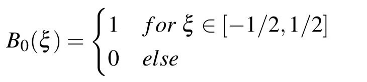
Knowing B0(ξ)spline

and its FT f0(t)

algebraic spline Bn(ξ)of arbitrary degree n and its FT fn(t)can be constructed in the following form:

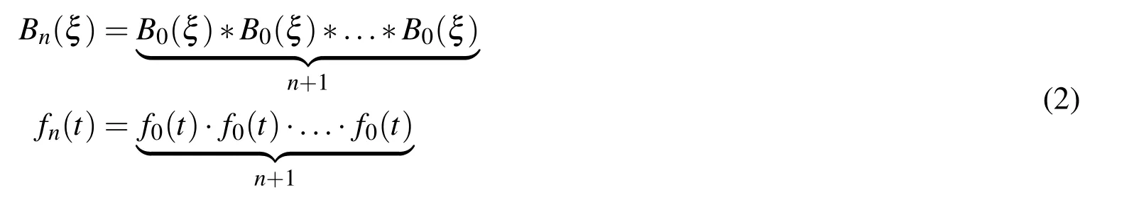
The function Bn(ξ)corresponds to the convolution of(n+1)B0(ξ)splines,so its support is a union of all supports of the convolution factors with the individual length h0=1.Thus,hn=(n+1)·h0.

Obviously,as the degree of polynomial n increases,the length of the function support increases too,and when n→∞,the corresponding length of the support hn∞.

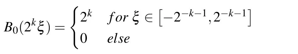
A modified form of the expression(1)is used for the function up(ξ)in[Gotovac(1986);Gotovac and Kozulic(2002)]in a way that B0(ξ)is summarized to half of its support length(h0/2);thus,a second member in the convolution is obtained,and then,this second member is again compressed to half of its support length(h0/4)and so on.

From the Paley-Wiener theorem[Gotovac and Kozulic(2002)]in the form(2nξ)dξ =1,it follows that the ordinates of each additional member are doubled.

Support of the function up(ξ)is the union of infinitely many segments,and yet,its length is finite

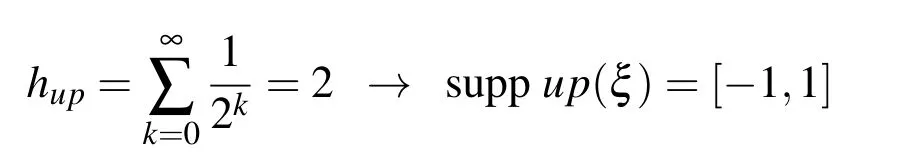
In[Gotovac(1986)],it is shown that the support length can be presented as a measure of the set of all binary rational poin√ts 2?k,k=0,1,...,∞,whereas all other points of the support likeform a set whose measure is-empty set.So,it is a compact support.

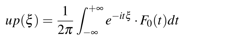
The consequence of repeated compression of the starting B0(ξ)spline to half its previous length increases the algebraic polynomial degree as shown in Fig.1.The FT of the basic atomic function up(ξ)according to(1),(2)and(3)is

From(4),using numerical procedures,it is possible to determine function values and the derivatives approximately according to formula

However,on the set of binary rational points

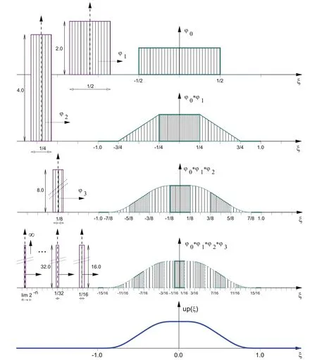
Figure 1:Basis function up(ξ)generation

The values and derivatives of the function up(ξ)can be determined in the form of rational numbers–i.e.,exactly.The function values at other points of the support are calculated with computer precision.

About ABF up(ξ)can be referred to as the perfect spline,which is differentiable an infinite number of times,although it is not an analytical function in any point of its support.Additionally,the finiteness is more expressive than in spline functions,and the smoothness is less than that for conventional basic functions such as algebraic and trigonometric polynomials.

The mother ABF up(ξ)maintains a good property of finiteness of B-splines and also possesses the important property of algebraic and trigonometric polynomials–the universality of the vector space UP that they form.

2.2 Differential functional equation for the function up(ξ)

The Fourier transform in the form of(4)can be converted to a form that is more suitable for describing the properties of the function up(ξ).F(t/2)is calculated from(4),and then the left side of equation(4)is divided by F(t/2),and the right side is divided bywhich gives

From the FT of function up(ξ)written in the form(6),it is obvious that up(ξ)possesses the quality of crushing(fragmenting);th?at is,any par?t of it contains the whole function(holographic effect).If sin(t/2)=eit/2?e?it/2/(2i)is substituted in(6)and the resulting equation is multiplied by(?1),after arranging,follows

On the left side of equation(8),there is a linear differential operator with constant coefficients,and on the right side,there is a linear combination of compressed and shifted ABFs up(ξ).

Fig.2 shows the function up(ξ)and its first derivative.It is evident that it is an even function and that its support is supp up(ξ)=[?1,1].

The support of the function up(ξ)is composed of two unit length characteristic intervals Δξ0.

Characteristic points ξkare the boundary points of characteristic intervals(the point of the origin and end points of the support ξ=±1).

The function value at the origin up(0)=1 is a consequence of the normed condition selection,which determines the value of the integral1 in the original domain or the value of the FT at the originin the image domain.

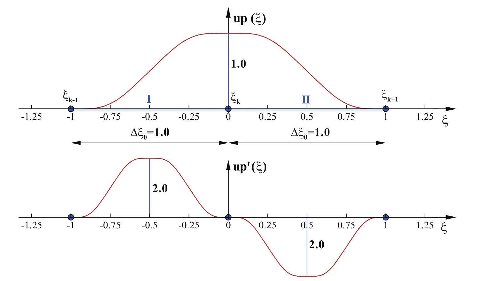
Figure 2:The function up(ξ)and its first derivative

2.3 Derivatives of the function up(ξ)

Derivatives of the degree greater than n of the up(ξ)function have a zero value at binary rational points(5).This means that the Taylor series at these points is finite and that the function up(ξ)for binary rational points coincides with a polynomial of nth degree,which is visible in Fig.1.

The first derivative can be represented as a linear combination of shifted and compressed functions up(ξ),as shown in equation(8).By differentiating the basic equation(8)and substituting the first derivative of the function up(ξ)with the right side of the starting equation(8),it is shown that the second derivative can also be presented as a linear combination of shifted and compressed up(ξ)functions:

By continuing the process of differentiation and replacing the first derivative from the basic equation,a general term for the derivative of the m-th degree is obtained:

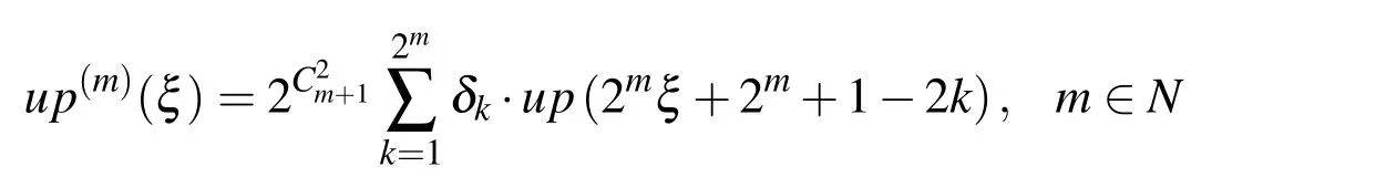
Figure 3 shows the function up(ξ),its first four and seventh derivative.It can be seen that the derivatives are made up of functions p(ξ),which are “compressed”on the interval with length 2?m+1and which have ordinates multiplied by a factor.A high degree derivative of the function up(ξ)when m → ∞ becomes a series whose individual member corresponds to Dirac’s function.

2.4 The value of the function up(ξ)at an arbitrary point

To calculate the values of the function up(ξ)at pointsit is necessary to know its values at pointsAccording to[Gotovac(1986);Gotovac and Kozulic(2002)]:

Given that the Taylor expansion of the function up(ξ)at binary rational points(5)represents a polynomial of the nth degree,a special order for calculating the value of the function up(ξ)at arbitrary point ξ ∈ [0,1]was proposed in[Gotovac(1986)]in the form:

where the coefficients Cjkare rational numbers that are determined according to the following formula:

Figure 3:Function up(ξ),the first four and the seventh derivative

2.5 Polynomial as a linear combination of shifted up(ξ)functions

An arbitrary function,as a linear combination of the shifted up(ξ)functions,can be written as:

where Δξn=2?nis a characteristic interval of the basis function.Particularly,if the coefficient Ckis an algebraic polynomial of mth degree of the index k,i.e.,

m=0,1,...,n,n∈N

then the function ?(ξ)from(10)is the algebraic polynomial of mth degree,whereas n denotes the greatest degree of the polynomial that is contained in a vector space UPn.

and after calculating the coefficientsfor the associated m according to(12)

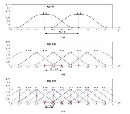
Figure 4:The basis function distribution for an accurate representation of the polynomials of 0,1 and 2 degrees

Using the coefficients(11)and(12)in the virtual domain and mapping the interval Δξnto the real length of the interval Δx,linear combination(10)in the real domain becomes

For example,algebraic polynomial P2(x)=a0+a1x+a2x2in the real domain is obtained using expressions(14)and(15)in the following form:

2.6 Vector space of functions UPn

Polynomials of the nth degree can be represented as a linear combination of basis functions obtained by moving the up(ξ)function.The individual basis function ?k(ξ)is obtained by moving the up(ξ)function on the abscissa axis for the value k·2?n,so that:

The exponent n determines the highest polynomial degree that can be accurately represented as a linear combination of basis functions ?k(ξ)according to(10).The coefficient k determines a displacement of the function up(ξ)with respect to the origin of the global coordinate system with the length of a characteristic interval Δξn=2?nso that it becomes a basis function ?k(ξ)(Fig.4.);thus,k has the role of a global index of the individual basis function.

As shown in Fig.4,for an accurate representation of monomials ξnon the interval of length 2?n,2n+1basis functions are required,so in this case,the dimension of vector space is dim(UPn)=2n+1.

For an accurate representation of monomials ξn+1,it is necessary to have 2n+2basis functions,so vector space UPn+1has a dimension of 2n+2.Therefore,the linear vector spaceUPn+1contains a spaceUPnbecause it is obtained by extending UPnspace with 2n+1linearly independent vectors,i.e.,displaced up(ξ)functions.Accordingly,as distinct from the space built out of basis splines,the function space UPnis universal,i.e.:

This fact makes it possible to form an iterative procedure in which the solution from the space UPnis used as a starting solution for searching the approximation in the space UPn+1.

2.7 Approximation of the function that is an algebraic polynomial

Let the given function be f(x)=?1+4x?2x2,x∈[0,1].We need to compute the approximation of the function using a linear combination of basis functions shown in Fig.4a,4b and 4c.

Using the collocation method,the system of equations and the corresponding approximation are obtained.

a)For two collocation points,the length of a characteristic interval is Δxa=1.The system of equations and the coefficientsCi,i=0,1 are:

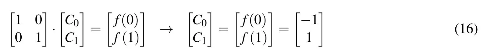
The approximation of the given function f(x)has the formefa(x)=C0·up(x)+C1·up(x?1)and is shown in Fig.5.

b)For three collocation points,the distribution of basis functions and collocation points are shown in Fig.4b.The length of a characteristic interval is Δxb= Δxa/2.There are five unknown coefficients and only three collocation points.When spline functions are used as an additional condition at the boundary,the first derivative is used so that there are double collocation points at the boundary.In the case of up(ξ)basis functions,we obtain the following matrix As:

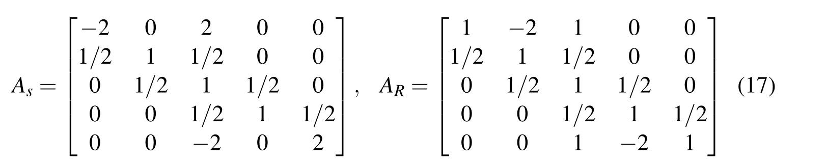
A system Asin(17)is singular.In[Rvachev and Rvachev(1979)],the system is preconditioned and solved by an iterative procedure.

The polynomials of the nth degree can accurately be described using the basis functions of the vector space UPnas shown in the previous section.However,in addition to ABF up(x),the vector space UPncontains the basis functions Fupn(x),[Gotovac(1986);Gotovac and Kozulic(2002);Rvachev and Rvachev(1979)],which can also exactly describe polynomials up to the nth degree.Basis function Fupn(x)is obtained as a result of a specific linear combination of up(x)functions.Additionally,a smaller number of basis functions is needed when accurately describing the polynomials of the nth degree on the characteristic interval than when using the up(x)functions.

Because all derivations over the order n in all points must be equal to zero,additional equations,instead of known derivatives on the boundary,can be written with the condition that the(n+1)th derivation of linear combinations of ABFs Fupn(x)in the middle of the first and the last characteristic intervals are equal to zero.

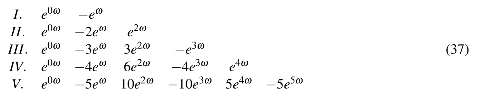
Additional equations at the beginning and the end of the matrix formally coincide with the corresponding operators of the finite differences.For the first five deriva-tions,the coefficients are as follows:

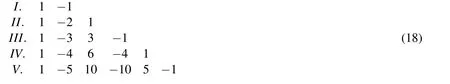
For distribution of basis functions formation according to Fig.4b(n=1),the second derivative must be equal to zero,so using(18)and replacing the first and the last line in(17),matrix Asbecomes a regular matrix AR.

c)Using the linear combination of ABFs distributed according to Fig.4c(n=2),the algebraic monomials of the zero,first and second degree and the polynomial obtained by their combination can be accurately described.Using the formula Δxc=Δxb/2=Δxa/4,the collocation method and additional equations from(18)the values of required coefficients are obtained.

The matrix for calculating the coefficients,which–multiplied by the corresponding basis functions from Fig.4c–accurately describe the given function,has the following form:

and the coefficients of the linear combination are

A linear combination of the basis functions shown in Fig.4c exactly describes a given function f(x)as shown in Fig.5.

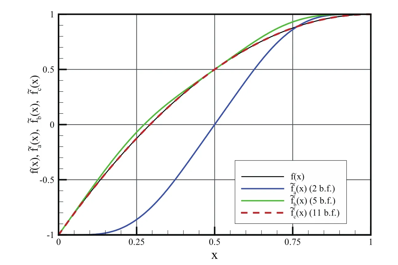
Figure 5:The function f(x)and its approximations

3 “Mother” function Eup(ξ,ω)of the exponential ABFs

3.1 Generation of the Fourier transform of the function Eup(ξ,ω)

The FT of the Eup(ξ,ω)function is constructed by a similar procedure applied on the up(ξ)function using the conditiondξ=1 on the corresponding compact support supp Eup(ξ,ω)=[?1,1].

Fig.6 shows a graphical representation of the generation process for the function Eup(ξ,ω)using the convolution theorem.In this procedure,the support lengths of exponential splines of the zero degree ?j(ξ,ω),j=0,1,2,...are reduced according to the law h=2?j:

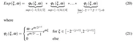
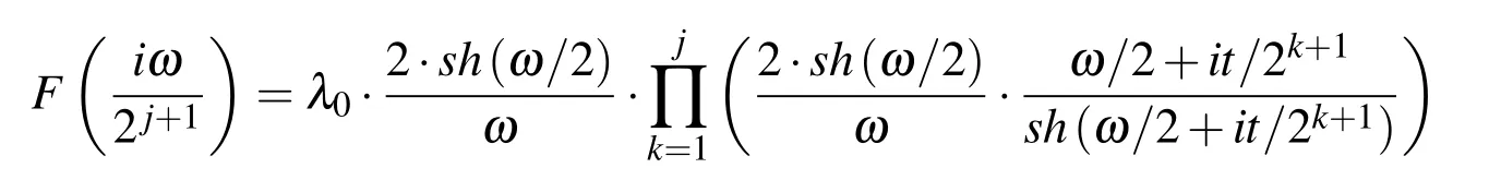
FT of the function Eup(ξ,ω)from(20)corresponds to the product of an infinite number of Fourier transformations of compressed splines of zero degree(21):

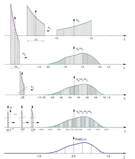
Figure 6:Exponential basis function Eup(ξ,ω)generation

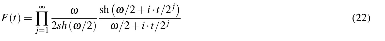
When the parameter ω approaches zero,expression(22)becomes expression(4).Hence,exponential ABF Eup(ξ,ω)becomes algebraic ABF up(ξ)when parameter ω becomes zero.The inverse FT or the function Eup(ξ,ω)itself,with the satisfaction of the normed condition,is:

By developing the right side of Eq.(23)in the Fourier series,the “original”of the function Eup(ξ,ω)can be determined.

The parameter ω has a role of frequency similar to trigonometric functions.Fig.7 shows that the function Eup(ξ,ω)is inclined to the left for negative values of the frequency ω＜0,whereas for positive values,it is inclined to the right.In the limiting case when ω → 0,the function Eup(ξ,ω)becomes up(ξ).Thus,the vector space EUP is denser than spaceUP andUP?EUP.

3.2 Differential functional equation for the function Eup(ξ,ω)

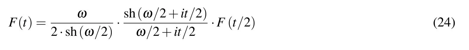
Differential functional equation for the function Eup(ξ,ω)is constructed from its known Fourier transform(22),which can be expressed in the following form:

In the following text,the basis function Eup(ξ,ω)will also be denoted as y(ξ,ω)due to shortness of the writing.

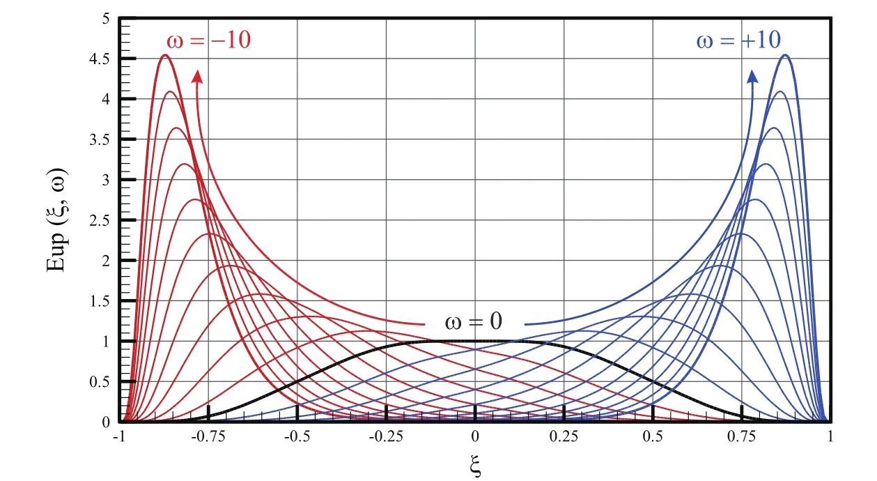
Figure 7:Function Eup(ξ,ω)for different values of parameter(frequency)ω

Multiplying equation(24)with ‘ω +it’and by short rearranging,the differential functional equation for the function y(ξ,ω)yields the final form

where the coefficients a and b are

In particular,when the value of the parameter ω=0,coefficients a=2,b=2,so that in this case,equation(25)is equivalent to equation(8).

The expression for the first derivative of y(ξ,ω)directly follows from equation(25)

3.3 Derivatives of the function Eup(ξ,ω)

Because on the left side of the differential functional equation(25)there is a member that contains a function y(ξ,ω),it is not possible,as it is in expression(8)for the up(ξ)function,to express derivations directly through the compressed functions on the right side of the equation.However,it is still achieved by applying the appropriate differential operator,[Gotovac(1986);Gotovac and Kozulic(2002);Rvachev and Rvachev(1979)],which converts the function y(ξ,ω)into a combination of derivatives from the zero to the m-th order:

On the right side of the expression,similar to the ABF up(ξ)(Fig.3),only a linear combination of compressed basis functions appears(Fig.8b).So,according to Eq.(27),the general form for an arbitrary derivative of the y(ξ,ω)function is determined by the following equation:

From expressions(28)–(30),it is obvious that the first derivative of the function y(ξ,ω)is the sum of two components.The first component(Fig.8a)is the zero derivative of the function y(ξ,ω)or the function itself multiplied by a coefficient,which in this case is just a parameter ω.The second component(Fig.8b)is a linear combination of compressed and displaced functions y(ξ,ω)similar to the first derivative of the function up(ξ).

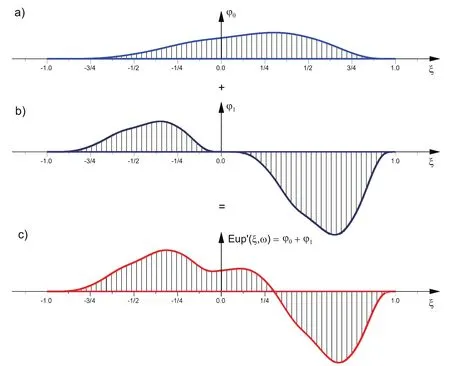
Figure 8:a)?0= ω ·y(ξ,ω),b)?1=a·y(2ξ +1)?b·y(2ξ?1),c)The first derivative of the function Eup(ξ,ω)

By continuing the process of derivation,it follows that the derivative of the function y(ξ,ω)of the mth order is obtained as a linear combination of the function derivatives up to the order(m?1)and the compressed and displaced function y(ξ,ω),similar to the mth derivative of the function up(ξ).

3.4 Relationship between basis functions Eup(ξ,ω)and exponential polynomials e2mωξ

By successive moving of just one finite basis function Eup(ξ,ω)along a real axis,the base of the vector space EUPnis formed.Arbitrary function ?(ξ)can be represented as a linear combination of functions from the vector space EUPn

For a linear combination(31)to represent an exponential monomial e2mωξ,it is necessary and sufficient that for the given n∈N and by applying a differential operator(27)on the expression(31),the linear combination on the right side is annuled.Hence,according to Eq.(28),it follows that the coefficients C(m)n(k)on the interval[k·2?n,(k+1)·2?n]must satisfy the following equation

The coefficients of linear combinationfrom Eq.(31)are the roots of the characteristic equation of linear recursion(32).

For example,for n=0(m=0)(Fig.9a),according to expression(32),the following recursion is obtained

Its solution is sought in the formFrom the corresponding characteristic equationis obtained.So,the exponential monomial of zero degreehas the final form

Analogously,for n=1(m=0,m=1),(Fig.9b),a linear recursion is obtained whose roots are

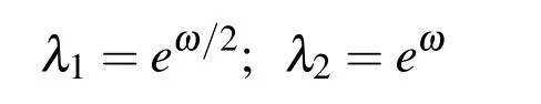
so the exponential monomials of the zero and the first degree can be expressed as a linear combination of the functions from the vector space EUP1in the following way

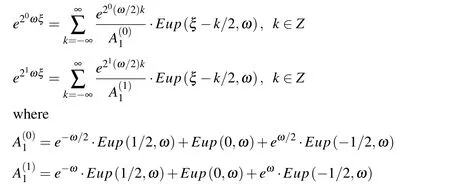
Generally,the exponential function e2mωξ,m=0,1,...,n,n ∈ N on the interval Δξn=2?ncan be accurately represented by a linear combination of 2n+1basis functions Eup(ξ,ω)mutually displaced by Δξnin the form the Eup(ξ?k2?n,ω)functions

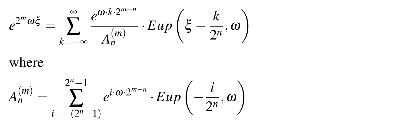
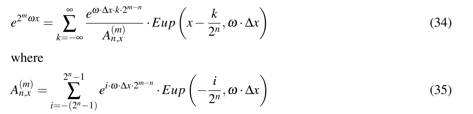
or in the real area of coordinate x:

So,a binary increase in the number of basis functions in the linear combination on the interval of length 2?nallows the development of an exponential function of degree m=0,1,...,n.

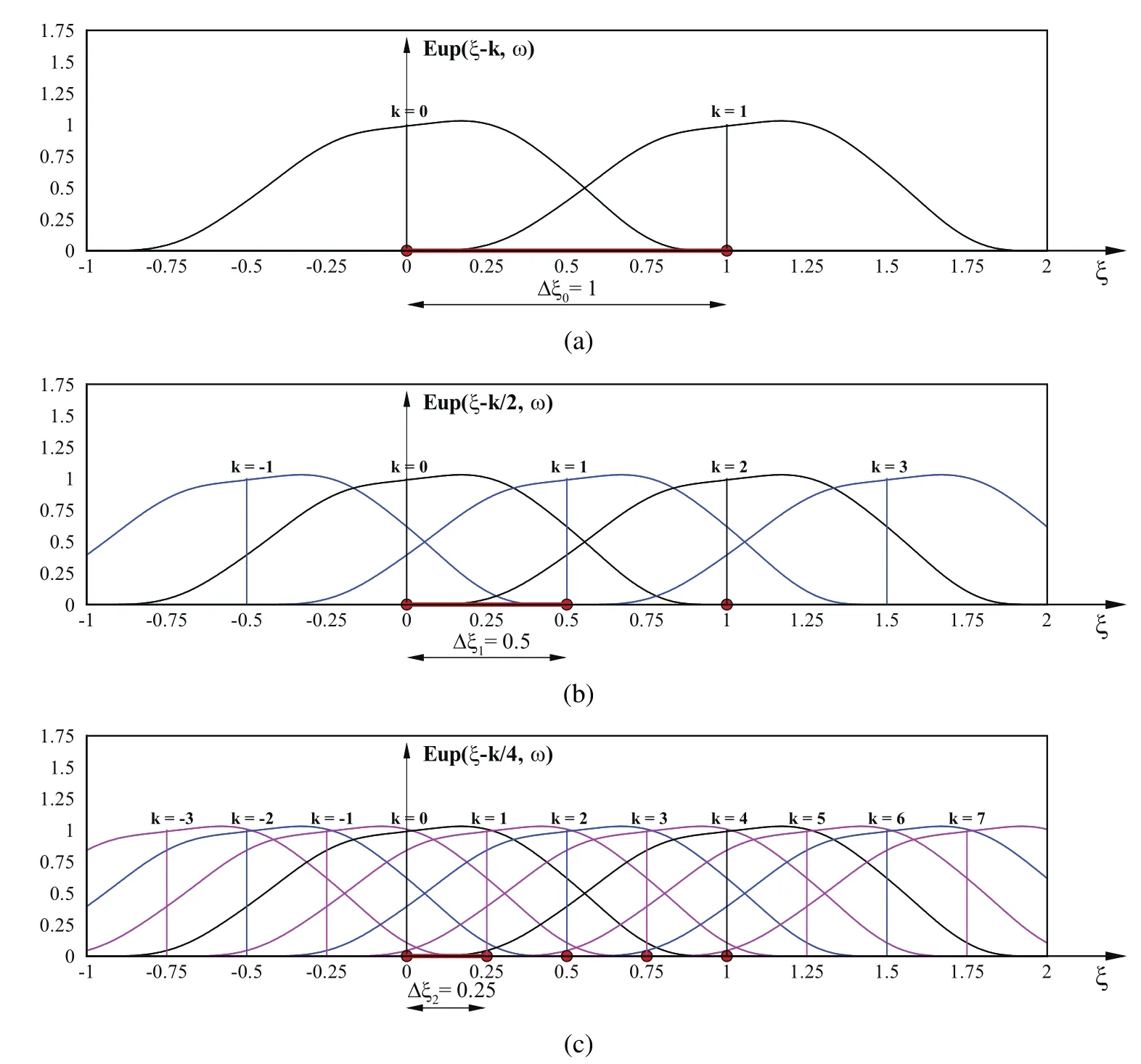
Figure 9:Development of exponential monomials of 0,1 and 2 degrees by

3.5 Example:Approximation of exponential polynomial function

The given function is f(x)= ?230 ·e0.6·x+304·e1.2·x?65·e2.4·x,x ∈ [0,1].Approximation of the function is sought in the form of a linear combination of basis functions shown in Fig.9a),9b)and 9c).

a)Using the collocation method and the associated frequency ωa=0.6 for Δxa=1,the system of equations and the coefficients Ci=1,i=0,1 are obtained:

Approximation of the function f(x)in the formefa(x)=C0·Eup(x,ωa)+C1·

Eup(x?1,ωa)is shown in Fig.10.

b)For three collocation points,the distribution of basis functions is shown in Figure 9b).The length of a characteristic interval is Δxb= Δxa/2,and the associated frequency is ωb=2·ωa=2·0.6=1.2.For three collocation points and two boundaries,conditional equations have a similar coefficient matrix as in Eq.(17).The obtained system is singular.The used vector space contains exponential polynomials up to the first degree.The first and the last equation should be replaced with the second derivative of EFup1(x,ω),[Gotovac(1986);Gotovac and Kozulic(2002);Rvachev and Rvachev(1979)],which are also contained in a vector space formed by the basis functions Eup(x,ω).For ABF,Eup(x,ω)can be written as alternative equations,similar to the approach described in Section 2.7 for ABF up(x)

When ω→0,the coefficients from(37)correspond to the coefficients in(18).The resulting approximationis shown in Fig.10.

c)The linear combination of ABF of exponential type arranged according to Fig.9c)accurately describes the exponential monomial of zero,first and second degree,or an exponential polynomial created by their combination.Using Δxc= Δxb/2=Δxa/4,the frequency ωc=21·ωb=22·ωa,the collocation method and additional equations from(37),the values of required coefficients are obtained.

The linear combination of basis functions shown in Fig.9c)exactly describes the given function f(x)as shown in Fig.10.

The linear combination of basis functions arranged with displacement Δx=h/4 accurately approximates any algebraic polynomial up to the second degree as shown in Section 2.7 because of the universality of the vector space.The same is valid for the exponential ABF.

So,for Δx=h/4=1/4 and frequency ω =2.4,exponential monomials e(2.4/4)·x,e(2.4/2)·x,e2.4·xand any of their linear combinations can be represented exactly.Thus,the given function f(x)fully coincides with approximatione fc(x)as shown in Fig.10.

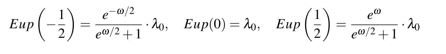
3.6 The values of the function Eup(ξ,ω)at the origin ξ=0 and ξbr

By integrating the differential functional equation(25)in the range from ξ = ?1 to ξ=0,[Gotovac(1986);Rvachev and Rvachev(1979)],the formula for numerically

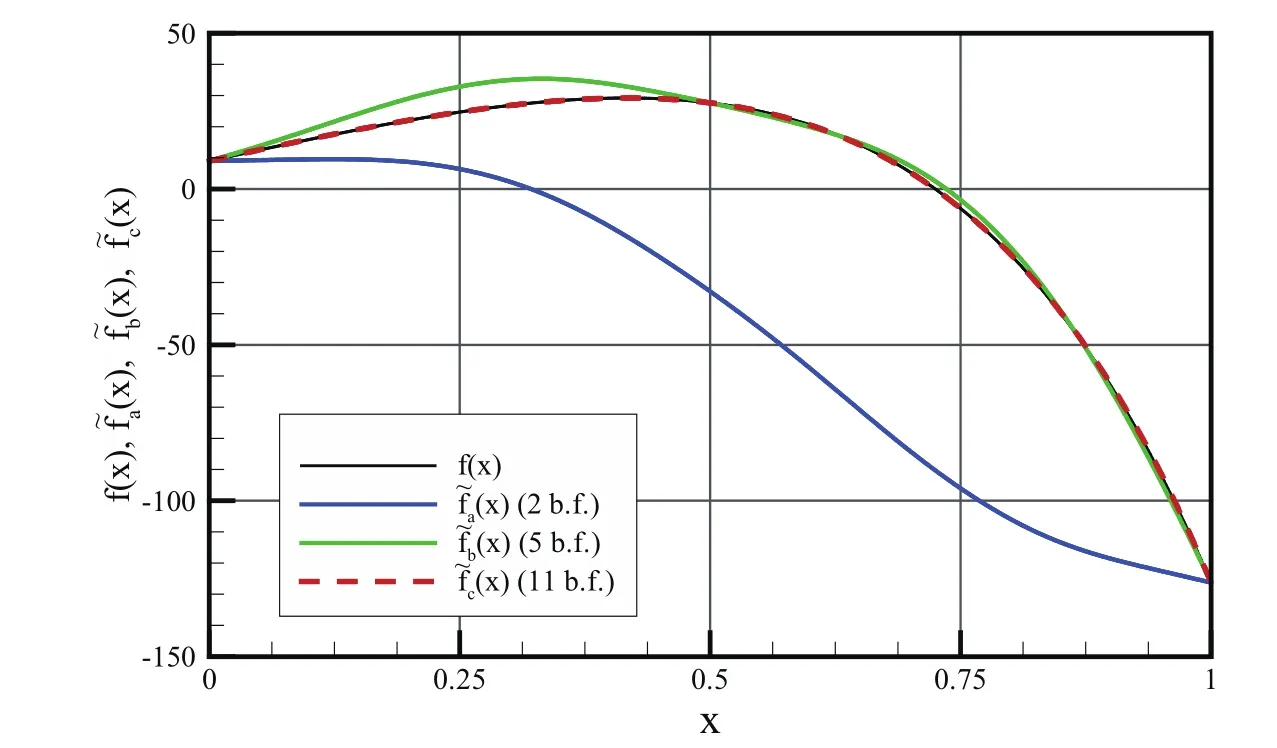
Figure 10:The function f(x)and its approximations

calculating the value of the function Eup(ξ,ω)at the origin is obtained:

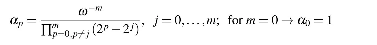
The expression for calculating the values of the function Eup(ξ,ω)in the binary rational points(5)is derived in Ref.[Rvachev and Rvachev(1979)]:

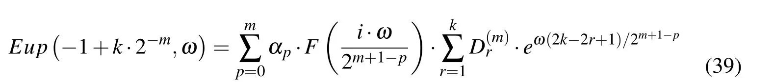
m=0,1,...,N;p=0,...,m;k=1,2,3...,2m+1;r=1,...,k

In this way,with(39),values of the function Eup(ξ,ω)in binary rational points ξbrcan be determined in a way that they depend only on the value of the function Eup(ξ,ω)at the origin ξ=0 from expression(38).

For example,the values of the function Eup(ξ,ω)at the binary rational points for m=1 are:

3.7 Values of the function Eup(ξ,ω)and the nth order derivatives at an arbitrary point

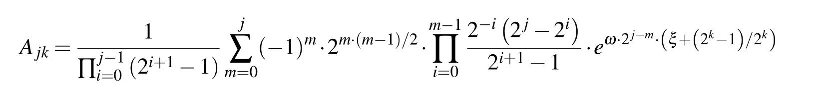
The value of the function Eup(ξ,ω)at an arbitrary point is determined by the series of a special form that is constructed based on the fact that the development of the function Eup(ξ,ω)into a Taylor series at the binary rational points ξbrcontains exponential polynomials analogous to the function up(ξ),which contains algebraic polynomials:

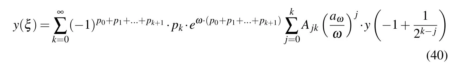
If the arbitrary point is displayed in binary form ξ=p0,p1,...,pk,where p0,p1,...,pkare the bits or digits 0 or 1 of the binary development of the coordinate ξ value,then the accuracy of the function Eup(ξ,ω)at an arbitrary point depends on the accuracy of an electronic computer.For that level of accuracy,a very small number of members in Eq.(40)are required.

It is understood that only the value at the origin λ0=Eup(0,ω)must be calculated numerically according to(38).

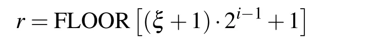
Using expressions(28)–(30)to(40),the expression for the nth order derivative of the function Eup(ξ,ω)at an arbitrary point is derived:

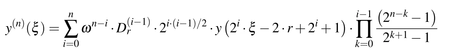
where n is the derivation order=1(by definition),whereas the coefficientsare defined by expressions(29)and(30),and r is an integer value defined by

4 ABF Eup(x,ω)implementation

4.1 Basis functions distribution

An ABF of exponential type in relation to the algebraic basis functions contains the parameter ω or,analogous to trigonometric functions,the frequency.

Vector space EUPnformed by ABF Eup(x,ω)with compact support supp Eup(x,ω)=[?Δx0,Δx0]has certain similarities to the vector space of trigonometric functions.Development of the unit value in both spaces is possible only in the case ω0=0,where

Function sinh(ω,x)=(eωx?e?ωx)/2 is composed of an exponential function with positive and negative frequencies.Thus,the vector space that contains the function sinh(ω,x)should also contain the basis functions with positive and negative frequencies,as in Fig.11b).

The odd indices are assigned to negative values of frequencies and even to positive ones.Approximation of a given function f(x),x∈[A,B],where the domain is divided into n intervals x0,can be described by a linear combination of basis functions Eup?x/?2kΔxk??i/2k,ωk

?mutually displaced per Δxk= Δx0/2kin the form:

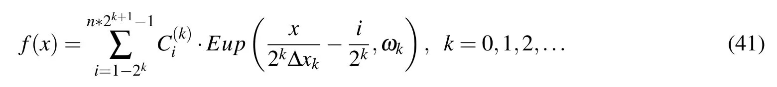
If k is finite,the function f(x)is approximated so that from the selected initial value x,the length of interval xkand the associated frequency ωkare determined.

Because the frequencies ωk,k=0,1,2,...are unknown in advance,it is necessary to choose a criterion and to construct an algorithm for the best frequency selection.The achieved accuracy of approximation ε(the difference between the given function f(x)and approximation?f(x))is compared with a given accuracy ε?,according to the following expression:

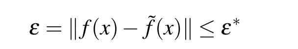
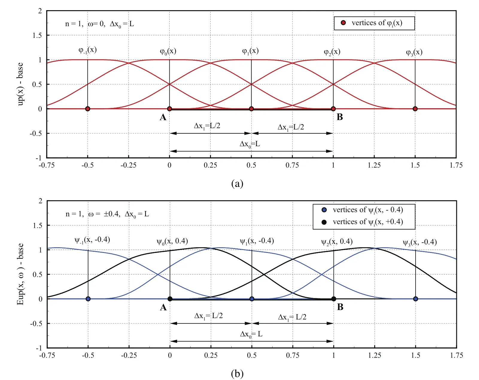
Figure 11:Distributions of the basis functions:a)up(x)and b)Eup(x,ω1)

The numerical procedure can be realized in different ways.Regardless of the approach,a global system of equations according to(41)is formed.The approximation can be searched for by the chosen number of basis functions and the associated frequency.Another way is based on the residuua method,in which a partial contribution of a particular frequency to an entire approximation is solved.Hence,a successive approximation of the difference between the given function and the current sum of the approximations of the residuua functions is performed.

The distribution of basis functions Eupi=?1,0,1,2,3 for frequency ω1= ?0.4 and the length of a characteristic interval Δx1=L/2 is shown in Fig.11b).

The basis functions are inclined to the right or to the left,depending on the sign of the frequency ω1.If the value of the frequency tends to zero,the basis functions become even and correspond to the algebraic ABFi= ?1,0,1,2,3 on Fig.11a).

4.2 Approximation of the given exponential function eωx

Let the function be given on segment AB in the formThe function approximations are searched using two characteristic intervals x and the basis functions distribution according to Fig.11b).The given function has an exponential character,and frequency ω has a value of 10(only positive values of frequencies).

Using the collocation method,coefficients=?1,0,1,2,3 of linear combinations of upbasis functions are calculated and presented in Table 1.

Coefficients Ciwith odd indices are equal to zero(see Table 1)because the corresponding basis functions do not contribute to the approximation.The given function has only positive frequency,so basis functions with a negative frequency must remain neutral so that the approximation is not spoiled.Approximation with the algebraic basis functions has a known oscillating character,whereas approximation obtained with exponential basis functions corresponds exactly to the given function.

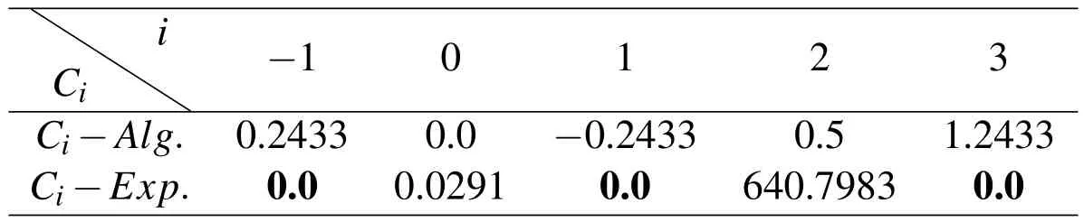
Table 1:Coefficients of the linear combinations

In general,the function to be approximated can include a frequency that is not known in advance by the sign or the value.Therefore,it is necessary to construct a method for determining the frequency of the basis functions Eup(x,ω)that gives the best approximation.

4.3 Determination of the best frequency

The approximation of the given function f(x)is searched using the collocation method in the form of a linear combination of exponential basis functions that contain an unknown frequency ω.

To determine the best frequency ω,it is necessary to calculate the eigenvalues ωi,i=1,2,...,n of the system matrix.For example,for a given function f(x)=?tgh((x?3/4)/0.02),x∈ [0,4]and selected interval Δx,five equations are obtained,and the eigenvalues of the corresponding coefficient matrix are illustrated on Fig.13.

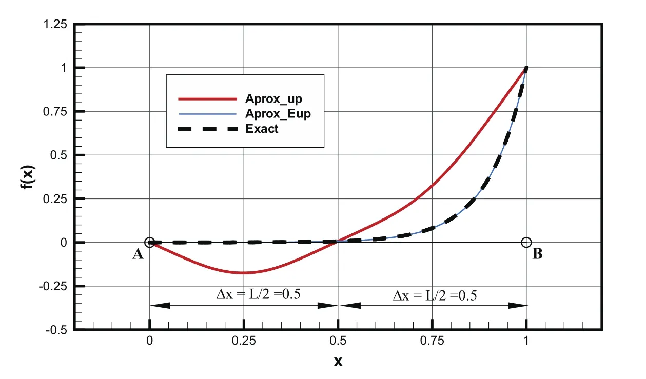
Figure 12:Comparison of approximations with the given function using algebraic and exponential basis functions with frequency ω=10

Hence,to determine the frequency ω that gives the best approximation,in a certain sense,appropriate additional criteria in the physical or some other sense,have to be chosen.

We selected the criterion of the least squares method for deviation between the given function and its approximation on each characteristic interval Δx:

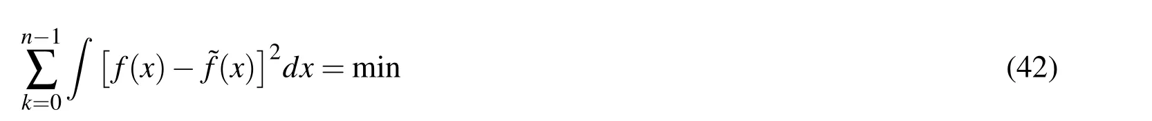
where f(x)is the given function,is an approximation of the function,and n is the number of characteristic intervals Δx in the domain AB.

Using Eq.(42),the frequencies ωi,i=1,...,5 are checked,and the one that gives the smallest square deviations is selected.

In this paper,a less economical though simpler method is selected.Generally,when the given function is not an algebraic polynomial or exponential function,the frequency step Δω is selected,and starting from zero,the value of the last square deviation of the approximation with respect to the given function is determined according to(42).

The dependence between deviation and the frequency of the basis functions is shown in Fig.14.The presented dependence is similar in the approximations of various functions.So,starting from zero,the deviation suddenly begins to rise and decline rapidly,thus achieving the local minima.

Figure 13:The roots of the frequency function ωi,i=1,...,5

The absolute minimum,if not registered at ω=0,is in the area of a very slight change of the deviation square dependent on ω,as shown in Fig.13.The linear combination of basis functions Eup(x,ω)with a calculated frequency ω ＞ 0 generally gives a better approximation than the analogous algebraic atomic functions.If the given function f(x)is a polynomial P1(x),the algorithm for determining the best frequency finds the value ω =0 because the deviation square is then LSS≡0,which corresponds to an absolute minimum.

Additionally,in the case of the exponential polynomials,e.g.,f(x)=e10(x?1),the best frequency ω =10 is obtained by the proposed algorithm because LSS ≡0,which determines the absolute minimum of the deviation square of the approximationfrom the given function f(x).

4.4 Approximation on the uniform grid

The function f(x)=TANGH((x?4/3)/0.02),x∈[0,4]is analysed.It is necessary to find an approximation by the linear combination of algebraic ABFs in the form of:

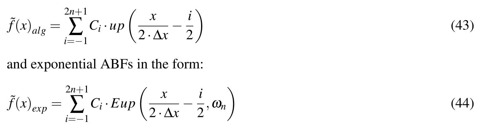
where n is the number of characteristic intervals on the length of the domain L=4.0,and i is the counter of the basis functions and collocation points except boundary points,which are double collocation points.

The numerical experiments were performed for the five different interval lengths Δx=L/n,where n=16,32,64,128,256.

A comparison of the given function and its approximations according to Eq.(43)is shown in Fig.14 in columns a1)–a5).

In the first four variants,the approximation oscillations are extremely expressive and are present even in the fifth variant for Δx=L/256.Oscillations occur when using any basis functions of the algebraic type.

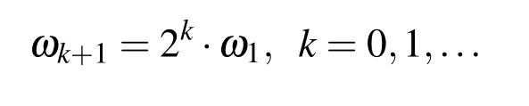
An attempt is made to eliminate the negative effect of the algebraic functions using basis functions of exponential type.Columns b1)–b5)in Figure 14 show the approximations according to(44)for the same resolutions as in columns a1)–a5).An incomparably better approximation can be seen.However,for each variant,the most appropriate frequency ω should be previously determined.The frequency ω is the same for all basis functions in the linear combination for selected number of intervals n according to(44).

According to the chosen criteria of least deviation squares between the approximation and the given function,the dependence between the deviation square and the frequency is shown in columns c1)–c5).

The algorithm for finding the best frequency is set only on the non-negative frequency values.If the frequency value is negative,it is controlled by the coefficients of the linear combination.

The effect of the exponential basis functions frequency impact on the approximation is visible already at n=8 in Fig.14 b1)with respect to a1).The frequency is directly related to the length of the interval Δx,and in all terms,the product Δx·ω appears.

The value of this product remains constant in all variants c1)–c5)and is approximately 2.243.In other words,it is sufficient to accurately calculate the frequency for the largest Δx,and for the smaller values of Δx,the frequency value isor in the case of diadic resolution increasing:

4.5 Approximation by levels(Multilevel Approximation)

Another approach to obtain approximations of the given function is a multilevel approach.We consider the function from the previous section.

In the zero step,the function approximatione f0(x)is subtracted from the given function f(x)=f0(x),and the new function f1(x)is obtained.Fig.15 b)compares the function f1(x)with a prescribed accuracy,for example,ε=±0.02.If accuracy is not satisfied,the approximatione f1(x)of the function f1(x)is searched(see Fig.

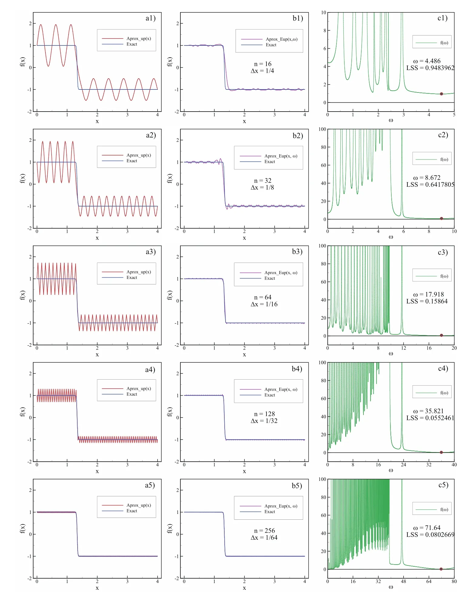
Figure 14:The approximations of the given function f(x):a1)–a5)by algebraic ABFs;b1)–b5)by exponential ABFs;c1)–c5)finding the minimum of the deviations square depending on the frequency ω

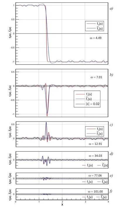
Figure 15:Given function f(x),function approximation?f(x)and residuua f(x)??f(x)by levels a)–f)

15 b)).Then,a comparison of the differenceand accuracy ε follows,and the procedure is repeated until it reaches the requested accuracy,as shown in Fig.15 f).

The final approximation of the function f(x)is obtained as the sum of the individual approximations at every level

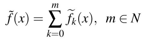
where the individual approximation is in fact a linear combination of the basis functions with corresponding frequency ωkdetermined according to the procedure described in Section 4.3:

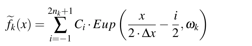
The starting grid n0is chosen arbitrarily,and the next is twice as dense,i.e.,n1=2·n0,or generally

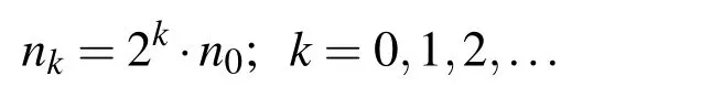
For example,in Fig.15,the initial grid n0=16 is used,and the corresponding frequency ω0=4.486 is calculated.

In this multilevel approximation method,approximately twice as many basis functions are needed than in the procedure using uniform grid described in Section 4.4 for the same accuracy of approximation.

However,this multilevel procedure is analogous to the procedure that is used in the adaptive Fup collocation method[Gotovac,Andricevic and Gotovac(2007)].In fact,at higher levels,only collocation points at which the residuum is higher than the prescribed accuracy are considered,whereas the other points do not have to be taken into consideration.Fig.15 shows that such a criterion leads to an adaptive procedure,which saves CPU time and drastically reduces the number of collocation points at higher levels.We leave the development of an adaptive procedure for the presented Eup basis functions to future research in the development of new non-stationary algorithms.Thus,in this section,each level is observed with all collocation points as a non-adaptive algorithm.

5 Conclusion

In this paper,the current knowledge regarding mother ABF function up(x)is once more synthesized.The approximation properties and expressions for the required mathematical operations are presented in a simpler,more understandable and userfriendly way.Using this approach,the basic atomic basis function of exponential type Eup(x,ω)is studied in detail[Gor?kov,Kravcenko and Rvacev(1994)].New expressions for calculating the values of the function,its derivatives and,of particular importance,the rules(elements)for its practical use are derived.The procedure for determining the frequency ω that gives the best approximation should especially be noted.The application of exponential ABF is shown in a few examples of the function approximations.The numerical results show excellent approximation properties of these basis functions,especially in the case of sharp gradient changes of the given function.Future research includes further development of the exponential ABF theory in the form of new EFup basis functions that will significantly improve the approximation properties of the Eup functions in the same way that algebraic Fup basis functions do for up functions.These more efficient exponential basis functions will be a basis for further development of the adaptive EFup collocation method,which can be applied in non-stationary problem algorithms of,e.g.,mass and heat conduction[Gotovac,Andricevic and Gotovac(2007)].

Atluri,S.N.;Han,Z.D.;Rajendran,A.M.(2004):A new implementation of the meshless finite volume method,through the MLPG “mixed”approach.CMES:Computer Modeling in Engineering&Sciences,vol.6,no.6,pp.491–514.

Atluri,S.N.;Shen,S.(2002):The meshless local Petrov-Galerkin(MLPG)method:A simple&lesscostly alternative to the finite element and boundary element methods.CMES:Computer Modeling in Engineering&Sciences,vol.3,no.1,pp.11–52.

Gor?kov,A.S.;Kravcenko,V.F.;Rvacev,V.L.(1994):Atomic exponential functions.UDK 517.95:518.517.

Gotovac,B.(1986):Numerical modelling of engineering problems by smooth finite functions.(In Croatian),Ph.D.Thesis,Faculty of Civil Engineering,University of Zagreb,Zagreb.

Gotovac,B.;Kozulic,V.(2002):On a selection of basis functions in numerical analyses of engineering problems.Int.J.Engineering Modelling,vol.12,no.1–4,pp.25–41.

Gotovac,H.;Andricevic,R.;Gotovac,B.(2007):Multi–resolution adaptive modelling of groundwater flow and transport problems.Adv.Water Resour.,vol.30,no.5,pp.1105–1126.

Gotovac,H.;Gotovac,B.(2009):Maximum entropy algorithm with inexact upper entropy bound based on Fup basis functions with compact support.J.Comp.Phys.,vol.228,pp.9079–9091.

Gotovac,B.;Kozulic,V.(2002):Numerical solving the initial value problems by Rbf basis functions.Int.J.Struct.Eng.Mech.,vol.14,no.3,pp.263–285.

Gotovac,H.;Kozulic,V.;Gotovac,B.(2010):Space-time adaptive fup multiresolution approach for boundary-initial value problems.CMC:Computers,Materials&Continua,vol.15,no.3,pp.173–198.

Han,Z.D.;Atluri,S.N.(2004):A Meshless Local Petrov-Galerkin(MLPG)approaches for solving 3-dimensional elasto-dynamics.CMC:Computers,Materials&Continua,vol.1,no.2,pp.129–140.

Iske,A.;K?ser,M.(2005):Two-phase flow simulation by AMMoC,an adaptive meshfree method of characteristics.CMES:Computer Modeling in Engineering&Sciences,vol.7,no.2,pp.133–148.

Kadalbajoo,M.K.;Patidar,K.C.(2002):Spline techniques for the numerical solution of singular perturbation problems.Journal of Optimization Theory and Applications,vol.112,no.3,pp.575–594.

Kozulic,V.;Gotovac,B.(2000):Numerical analyses of 2D problems using Fupn(x,y)basis functions.Int.J.for Engineering Modelling,vol.13,no.7.

Kozulic,V.;Gotovac,H.;Gotovac,B.(2007):An adaptive multi-resolution method for solving PDE’s.CMC:Computers,Materials&Continua,vol.6,no.2,pp.51–70.

Kozulic,V.;Gotovac,B.(2011):Elasto-plastic analysis of structural problems using atomic basis functions.CMES:Computer Modeling in Engineering&Sciences,vol.80,no.4,pp.251–274.

Kolodyazhny,V.M.;Rvachev,V.A.(2007):Atomic functions:Generalization to the multivariable case and promising applications.Cybernetics and Systems Analysis,(KhAI),Kharkov,Ukraine.vol.43,no.6,pp.893–911.

Konovalov,Y.Y.;Kravchenko,O.V.(2014):Applicationof newfamily ofatomic functions cha,nto solution of boundary value problems.Days on Diffraction,IEEE.

Kravchenko,V.F.;Rvachev,V.A.;Rvachev,V.L.(1995):Mathematical methods for signal processing on the basis of atomic functions.Radiotekhnika i Elektronika,vol.40,no.9,p.1385.

Kravchenko,V.F.;Basarab,M.A.;Perez-Meana,H.(2001):Spectral properties of atomic functions used in digital signal processing.J.Commun.Technol.Electron.,vol.46,pp.494–511.

Libre,N.A.;Emdadi,A.;Kansa,E.J.;Shekarchi,M.;Rahimian,M.(2009):Wavelet based adaptive RBF method for nearly singular poisson-type problems on irregular domains.CMES:Computer Modeling in Engineering&Sciences,vol.50,no.2,pp.161–190.

Lin,H.;Atluri,S.N.(2000):Meshless local Petrov-Galerkin(MPLG)method for convection-diffusion problems.CMES:Computer Modeling in Engineering&Sciences,vol.1,no.2,pp.45–60.

Mai-Duy,N.(2004):Indirect RBFN method with scattered points for numerical solution of PDEs.CMES:Computer Modeling in Engineering&Sciences,vol.6,no.2,pp.209–226.

McCartin,B.J.(1981):Theory,computation,and application of exponential splines.Courant Mathematics and Computing Laboratory,Research and Development Report.

Prenter,P.M.(1989):Splines and variational methods.New York,Wiley.p.323.

Radunovic,D.(2008):Multiresolution exponential B-splines and singularly perturbed boundary problem.Numer.Algor.,vol.47,pp.191–210.

Rvachev,V.L.;Rvachev,V.A.(1971):On a finite function.Dokl.Akad.Nauk Ukr.SSR,vol.A,no.8,pp.705–707(in Russian).

Rvachev,V.L.;Rvachev,V.A.(1979):Nonclassical methods of approximation theory in boundary value problems.Naukova Dumka.Kiev.

Shen,S.P.;Atluri,S.N.(2005):A tangent stiffness MLPG method for atom/continuum multiscale simulation.CMES:Computer Modeling in Engineering&Sciences,vol.7,no.1,pp.49–67.

?arler,B.(2005):A radial basis function collocation approach in computational fluid dynamics.CMES:Computer Modeling in Engineering&Sciences,vol.7,no.2,pp.185–193.

Vasilyev,O.V.;Paolucci,S.(1997):A fast adaptive wavelet collocation algorithm for multidimensional PDEs.J.Comput.Physics,vol.125,pp.16–56.

Zienkiewicz,O.C.;Taylor,R.L.;Zhu,J.Z.(2013):The Finite Element Method:Its Basis and Fundamentals,Butterworth-Heinemann,Seventh Edition.

1Faculty of Civil Engineering,Architecture and Geodesy,University of Split,Matice hrvatske 15,21000 Split