Geodynamic evolution of the Earth over the Phanerozoic: Plate tectonic activity and palaeoclimatic indicators

Christian Vérard, Cyril Hochard, Peter O. Baumgartner, Gérard M. Stampfli

Université de Lausanne (UNIL), Institut des Sciences de la Terre (ISTE), Geopolis, CH-1015 Lausanne, Switzerland

Abstract During the last decades, numerous local reconstructions based on field geology were developed at the University of Lausanne (UNIL). Team members of the UNIL participated in the elaboration of a 600 Ma to present global plate tectonic model deeply rooted in geological data, controlled by geometric and kinematic constraints and coherent with forces acting at plate boundaries.In this paper, we compare values derived from the tectonic model (ages of oceanic floor,production and subduction rates, tectonic activity) with a combination of chemical proxies(namely CO2, 87Sr/86Sr, glaciation evidence, and sea-level variations) known to be strongly influenced by tectonics. One of the outstanding results is the observation of an overall decreasing trend in the evolution of the global tectonic activity, mean oceanic ages and plate velocities over the whole Phanerozoic. We speculate that the decreasing trend reflects the global cooling of the Earth system. Additionally, the parallel between the tectonic activity and CO2 together with the extension of glaciations confirms the generally accepted idea of a primary control of CO2 on climate and highlights the link between plate tectonics and CO2 in a time scale greater than 107 yr. Last, the wide variations observed in the reconstructed sea-floor production rates are in contradiction with the steady-state model hypothesized by some.

Key words geodynamic, plate tectonics, plate model, Phanerozoic, palaeoclimate, CO2,strontium, glaciation

1 Introduction*

The spatial and temporal distribution of continents and oceans throughout the Phanerozoic is of major concern in a wide range of scientific studies. At the interface between the inner and the outer shells, lithospheric plates are an es?sential link of the global Earth system. On the one hand,palinspastic reconstructions offer an ideal framework to geological and palaeogeographical studies; on the other hand, they can be used as boundary conditions in palaeocli?matic, palaeoceanographic and mantle circulation models.

By assembling the regional?scale tectonic reconstruc?tions developed at the University of Lausanne (UNIL) dur?ing the last 20 years (Stampfliet al., 1991, 1998, 2001,2002a, 2002b, 2003, 2011, 2013; Stampfli, 1993, 2000;Stampfli and Pillevuit, 1993; Stampfli and Borel, 2002,2004; Stampfli and Kozur, 2006; von Raumeret al., 2006,2009; Bagheri and Stampfli, 2008; Ferrariet al., 2008;Moixet al., 2008; von Raumer and Stampfli, 2008; Flores-Reyes, 2009; Stampfli and Hochard, 2009; Wilhem, 2010;Vérardet al., 2012a; Vérard and Stampfli, 2013a, 2013b;von Raumeret al., 2013), we have created a global plate tectonic model covering the whole Earth’s surface (i.e.,continental and oceanic realms) over the Phanerozoic Eon. Initially presented in Stampfli and Borel (2002) and Stampfli and Borel (2004), the “dynamic plate boundaries”method then used to develop the model has been updated in the light of new studies and techniques.

The model presented herein corresponds to the model developed at UNIL, and purchased by Neftex Petroleum Consultant Ltd. in January 2010; it is therefore hereafter referred to as the UNIL model (v.2011, ? Neftex). It is beyond the scope of the present paper to discuss the va?lidity of each field study interpretation and the reader is asked to refer to the aforementioned papers for all the de?tails. We focus upon: (1) further detailing the method and techniques employed to develop the global plate tectonic reconstructions; (2) comparing a series of tectonic factors stemming from the model with various proxies thought to reflect variations in plate tectonics, namely: mean oce?anic ages and plate velocities versus sea?level variations,tectonic activity versus CO2and markers of glaciation ex?tent, and length of collision zones and87Sr/86Sr (Sr?ratio)isotopic changes. The goal is twofold: (1) validating the robustness of the model and (2) better comprehending the relationship between tectonics and such palaeoclimatic in?dicators. Using an innovative way to convert 2D maps into 3D topographic surfaces, the robustness of the model is tested more directly against sea?level and Sr?ratio varia?tions in another paper (Vérardet al., 2015).

2 Method — From geodynamic units to tectonic plates

To reconstruct the Earth's history, we developed an ap?proach in which the elementary units are named geody?namic units (GDUs; see definition below). Using geologi?cal data of geodynamic interest (i.e., providing insights on geodynamical environments such as rift zone, passive margin, active margin, collision zone,etc.), the geological histories of GDUs are correlated through space and time to define larger scale geodynamic scenarios. In turn, the regional geodynamic scenarios are correlated to generate global scale plate tectonic models.

In plate tectonic modeling, the lithosphere is divided into smaller entities usually named “terranes”. However,the latter term was used long before the advent of plate tectonics (d'Aubuisson de Voisins, 1819; Dana, 1863;Schardt, 1893) and his fundamental meaning has been a matter of hot debate (e.g., Seng?ret al., 1990; Howell,1995; Le Grand, 2002). As stated by Howellet al.(1985),a terrane is frequently defined as “a fault bounded package of rocks of regional extent” but we do think that such ac?ceptance is far too imprecise and often leads to confusion.To avoid misunderstandings and supersede the term “ter?rane”, we introduce the term “Geodynamic Unit” (GDU).A GDU describes the present?day smallest continental/oceanic fragment that underwent the same geodynamic evolution since 600 Ma (starting age of the model). The Earth’s history is reconstructed by redistributing the GDUs through space and time. The GDUs position is controlled by palaeogeographic data (e.g., palaeoclimatology, pal?aeobiogeography, palaeomagnetism; see below) associ?ated with geological data of geodynamic interest. A GDU is a spatial object used to carry information from present to past and is thus only a geological marker. GDUs are defined in the present-day configuration and keep their ini?tial shape through time. Consequently, geological bending,stretching or shortening is not corrected within a GDU,but tight (untight) fits are used not to underestimate crustal extension (shortening). A map of GDUs as defined in the UNIL model (v.2011, ? Neftex) is shown in Figure 1.

Geodynamic scenarios are usually represented as 2D cross?sections of regional scale (see an example in Figure 2). They are designed to account for the geological history of each GDU involved, and to respect physical parame?ters known to govern plate tectonics. As generally agreed(e.g., Forsyth and Uyeda, 1975; Zhong and Gurnis, 1995;Anderson, 2001; Conrad and Lithgow?Bertelloni, 2002;Stern, 2004; Schellartet al., 2007), we do consider that forces acting on plate boundaries (i.e., slab pull, slab roll?back and ridge push) are the primary drivers of plate tec?tonics. Any change in plate motion must then be related to evolution of the boundary conditions. We stress that plate boundaries are lithospheric discontinuities which cannot appear spontaneously by themselves. In the UNIL model(v.2011, ? Neftex), new plate boundaries can be created in the following configurations:

In extension: (1) lithospheric plate under extension can undergo rifting in its continental part because of the rheo?logical weakness of the middle crust (e.g., Cloos, 1993).A present-day example of such configuration is the Red Sea opening; (2) due to slab roll?back, arcs are also zones of weakness where extension may occur. In this case, the former ridge ceases and jumps into the arc. The latter splits into an abandoned arc and a new active arc (e.g., the Lau ridges/Tonga?Kermadec active arc or the Marianas).

In convergence: (1) subduction can initiate if a lith?ospheric discontinuity pre?exists such as ridge failure and transform fault failure (e.g., McKenzie, 1977; Mueller and Phillips, 1991; Mülleret al., 1998; Baeset al., 2011a); (2)subduction propagation and subduction reversal (i.e., re?vival of subduction behind the accreted terrane after colli?sion in forward or reverse direction respectively) together with step faults (Baeset al., 2011b) are the only processes that can turn a passive margin into an active margin. Con?tinued aging of a passive margin alone, in particular, does not result in conditions favorable for transformation into an active margin (Cloetinghet al., 1982, 1984).

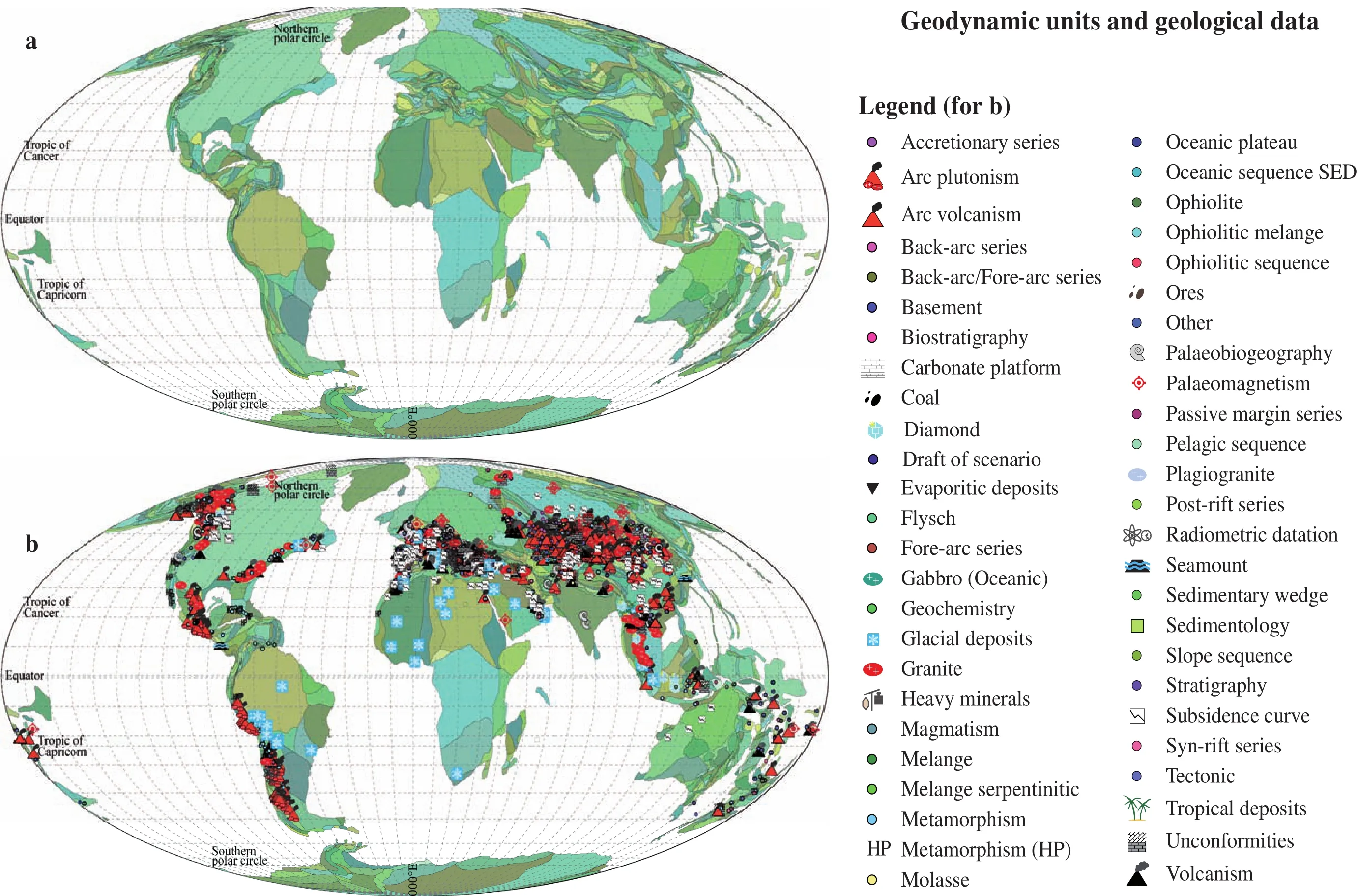
Figure 1 Geodynamic units and geological data of the UNIL model (v.2011; ?Neftex). a-Geodynamic unit map of the world including 1046 entities (mainly continental, except in the Mediter?ranean, Caribbean and peri?Australian areas). Colors have been arbitrary attributed to each GDUto distinguish them one from the other, but have no meaning; b-Spatial distribution of 2897 among more data used in the model to constrain past reconstructions. The legend details the 50 possible types of geological data (see Hochard, 2008 for further discussion).

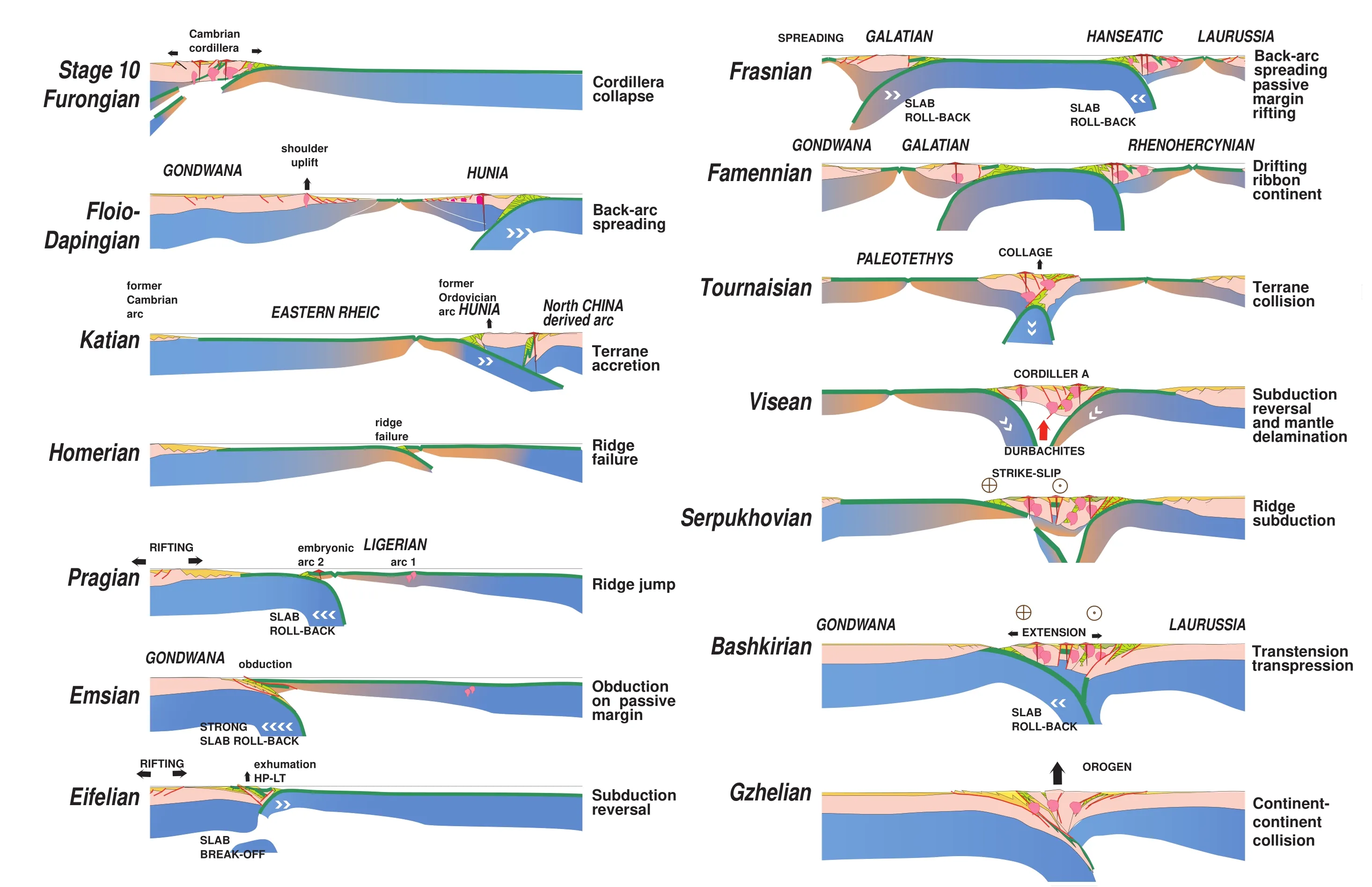
Figure 2 Example of geodynamic scenario after Stampfli et al. (2011; op.cit. Figure 2). Geodynamic scenarios are usually represented as cross sections. Here, a model of the evolution of the Gondwana margin from latest Cambrian (Stage 10; Furongian) to latest Carboniferous (Gzhelian; Upper Pennsylvanian). The sections are tied to Gondwana (left), so the continent to the right is changing through times. For the left part of the figure NorthChina elements are facing Gondwana, whereas for the right side of the figure it is Laurussia. The horizontal scale is not respected.

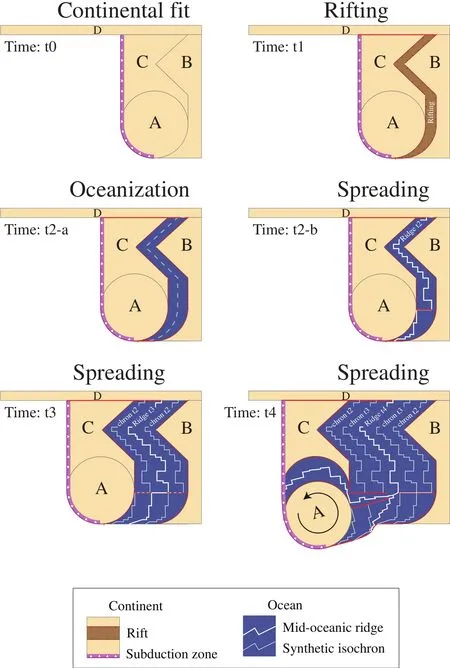
Figure 3 Technique used for the reconstructions, with in particular, definition of synthetic ridge and isochrons in disappeared oceans.See details in text.

To avoid unrealistic velocities, we arbitrarily limit plate velocity to a maximum of 22 cm·yr-1. This value corre?sponds to the present?day highest equatorial plate velocity on Earth after DeMetset al.(1994). This value is of course subject to caution and was more used as warning sign dur?ing reconstruction; however, we did not need to strictly use this parameter to constrain the model.

A lot of reconstruction models are actually not con?structed using plate tectonic principles but with an ap?proach akin to continental drift. They use continental blocks (i.e., similar to our GDUs) as individual entities moving their own way without paying enough attention to the plate in which the blocks are included. Although they have disappeared, past plate boundaries can be retrieved thanks to geological data. In the UNIL model (v.2011, ?Neftex), a tectonic plate is an assemblage of GDUs fully surrounded by plate boundaries forming an interconnected network. Except in plate boundary areas, a tectonic plate is considered as an undeformable rigid body. No feature constituting a plate (in particular no GDU) can move its own way. This approach offers a strong control on plate motion since any data of a GDU belonging to a given plate helps to define the location of the entire plate. The mo?tion of plates is controlled by the geodynamic scenarios.Knowing the positions of the GDUs and the timing of ma?jor geodynamic events (e.g., continental break?up, colli?sion, subduction initiation or reversal,etc.), one can trace the motion of plates.

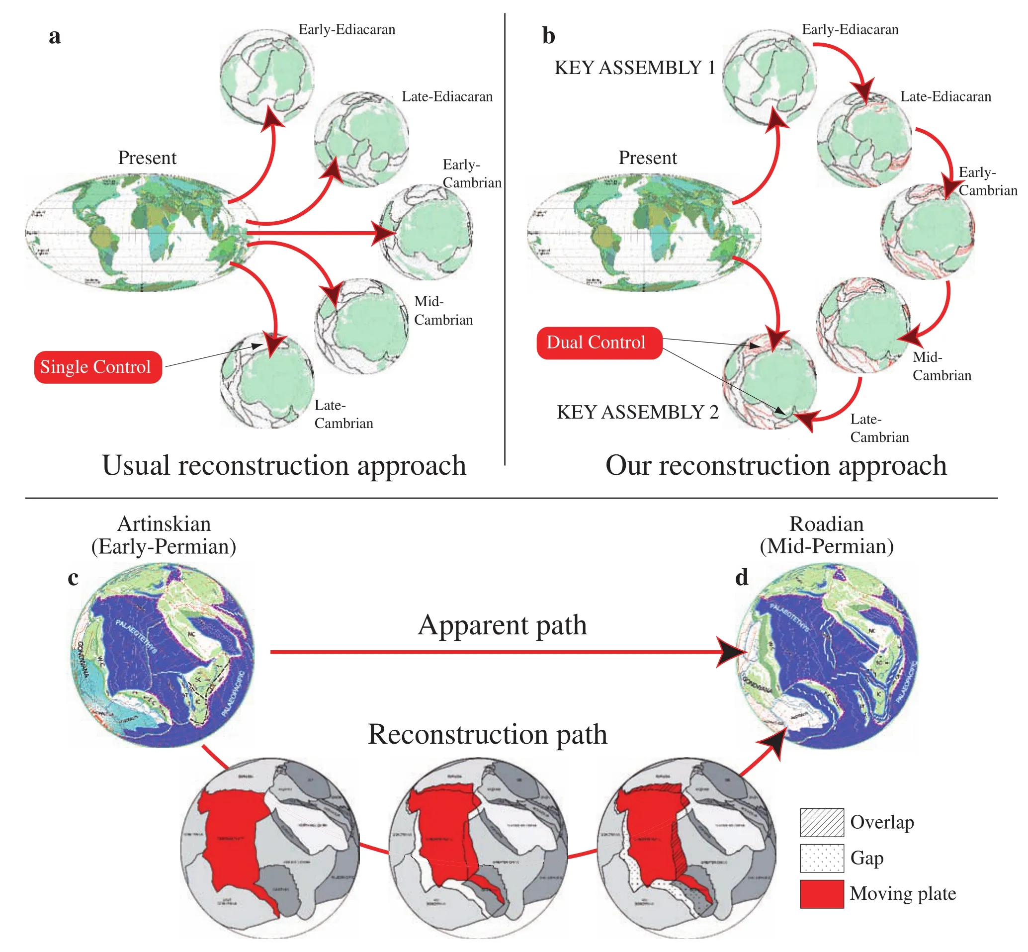
Figure 4 Comparison between the usual reconstruction approach and our approach. a-In the usual approach, the present?day conti?nents are divided into blocks redistributed using palaeomagnetic data and palaeobiogeographic data available for each age; b-In our approach, the continental blocks (GDUs) are redistributed to form key assemblies (for which palaeomagnetic and palaeobiogeographic data are known and reliable) but the in?between time frames are reconstructed following geodynamic scenarios based on other geologi?cal data. Key assemblies are thus controlled twice. The coherence of the geological history is as important (if not more) as the raw data which often suffer large uncertainties; c and d-Detailed steps between two reconstructions. Plate positions are interpolated to go from c to d. As the plate polygons are preserved, overlaps and gaps can be identified which lead to the definition of new converging (i.e.,subduction or collision zones) or diverging (i.e., ridges and rifts) plate boundaries. Reconstructions from Atinskian (mid?Cisuralian;Early Permian) to Roadian (early?Guadalupian; Middle Permian) after Ferrari et al. (2008). This figure is in part derivative from the Neftex Geodynamic Earth Model, ? Neftex Petroleum Consultants Ltd., 2011.

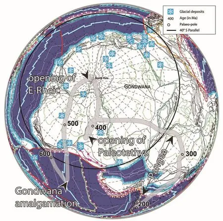
Figure 5 Apparent polar wander path for Gondwana after Stampfli et al. (2013; op.cit. Figure 5). 300 Ma to present?day palaeo?poles are from Torsvik and van der Voo (2002); Frasnian (early Late Devonian) to 300 Ma palaeo?poles are from Torsvik and van der Voo(2002). Older segments of the path are based on two key poles (at ca. 550 Ma and ca. 480 Ma) consistent in the studies of Schmidt et al. (1990), Bachtadse and Briden (1991), Li and Powell (2001), Torsvik and van der Voo (2002) and McElhinny et al. (2003). In the intervals, following the same approach as in Scotese and Barrett (1990), the pole locations are constrained using the global distributions of carbonates and glacial deposits. The present figure shows an example for Hirnantian time. Additionally we minimized the resulting velocity of Gondwana to keep a value near 8 cm·yr-1 comparable with its velocity between 300 Ma and 0 Ma. This figure is in part derivative from the Neftex Geodynamic Earth Model, ? Neftex Petroleum Consultants Ltd., 2011.

For mid?oceanic ridges, for instance, the location and geometry are inferred from the global isochrons dataset of Mülleret al.(2008a) where possible. For disappeared oceans, the exact shape of mid?oceanic ridges is not known, and will never be. However, during the continental break?up, if plate velocities and geometries are known, the space between the detaching and the left?over fragments(into which the new ridge formed) is constrained. As an example, Figure 3 shows how a continental block com?posed of two GDUs (A and B) is detached from GDU C at time t1. According to the geodynamic scenario estab?lished for these GDUs, the timing of the oceanization (in the sense of the presence of oceanic crust and/or denudated mantle) and the velocity are known (Figure 3; time t2?a).In the available space, a new ridge is designed (Figure 3;time t2?b) with transform segments following small circles of the rotation. From time t2 to time t3, the ridge becomes two symmetric synthetic isochrons, which strongly con?strain the position of the next ridge. At time t4, the rotation of GDU A is then constrained by the plate geometry, in particular by the space for the triple junction to develop and by the spreading rate on the other side of the mid?oceanic ridge formed between A and C. By preserving the synthetic isochrons step after step, the uncertainties are re?duced and the oceans are reconstructed.

The reconstruction work is carried out from past to pre?sent. Starting hitherto with a continental assemblage at 600 Ma, crustal material is added/removed in divergent/con?vergent areas marked by newly defined plate boundaries.From one reconstruction to the next, plate positions are interpolated and former plate polygons are first preserved to identify the diverging (gaps) and converging (overlaps)areas (Figure 4c and 4d). As for mid?oceanic ridges, new plate boundaries (i.e., subduction zones, collision zones or transform faults) are defined in those restricted areas, lim?iting the uncertainties and ensuring the continuity in the model.

This approach is based on the relative movements of plates constrained by the GDUs. For major continental blocks (i.e., Baltica, Laurentia, Siberia and Gondwana),published apparent polar wander paths (Torsviket al.,1996, 2008; Torsvik and van der Voo, 2002; Torsvik and Cocks, 2005; Cocks and Torsvik, 2007) were used and sometimes modified to fit palaeogeographic data and/or limit the velocity of the reference plate (see Figure 5 and Hochard, 2008 for further details). However, palaeo?poles are not sufficient as (1) they give no constraint in palaeolongitude (except in Torsviket al., 2008); (2) they are of?ten subject to large uncertainties; (3) most of the time, they do not exist for smaller GDUs. To overcome this issue, we employed the trial?and?error method and performed nu?merous iterations. Like Scoteseet al.(1999), we followed palaeogeographic principles and try to distribute GDUs thanks to rock deposits providing palaeoclimatic indi?cations (e.g., carbonates, evaporates, limestones, coals,tillites,etc.). Following Cocks and Torsvik (2002) for in?stance, we additionally use palaeo?faunas. But rather than trying to locate a continental block on the basis of a single study at all ages, we select key ages where palaeomag?netic, palaeoclimatic and palaeobiogeographic data are in good agreement for many blocks and define “key assem?blies” (Figure 4b). In between frames are reconstructed following geodynamic scenarios. Supplementing the pal?aeomagnetic, palaeoclimatic and palaeobiogeographic data with a geodynamically consistent history offers an additional constraint (“dual control” in Figure 4b) which,in our opinion, represents a major step forward.

3 Geodynamic model and derivative maps

The UNIL model (v.2011, ? Neftex) comprises 48 re?constructions extending back to 600 Ma every 5 Ma to 20 Ma (Figure 6a). On average, a reconstruction is made up of about 1700 features (lines, points, polygons under ArcGIS?) of 26 possible types describing the geodynamic context (e.g., collision zone, mid?oceanic ridge, passive margin) or the palaeogeography (e.g., basin limit, geo?graphical marker) (see legend in Figure 9a). The model is based on 1046 GDUs associated with 2897 geological data distributed throughout the Phanerozoic (Figure 1 and temporal distribution in Figure 6b). A reconstruction is constrained on average by 267.4 geological data of 50 possible types (see legend in Figure 1 and Hochard, 2008 for further discussion) with a minimum of 86 data points at 6 Ma and a maximum of 481 data points at 330 Ma.At 600 Ma (first reconstruction), 83% of the Earth surface is reconstructed. This value rises gradually to reach 100%as early as 461 Ma (black squares in Figure 6a). The first reconstruction includes 509 GDUs only. However, once a GDU is present (i.e., comes into existence) on a recon?struction, it is preserved and evolves to end up in its final present?day position. Consequently, the amount of GDU rises progressively according to the geological history(black line in Figure 6a). The smallest GDU is 0.183×103km2large, and the largest is 1.65×107km2large (Figure 7). For comparison, the widespread Earthbyte Plate Model 2009 (online data: http://www.earthbyte.org/Resources/earthbyte_plate_model_2009.html; Mülleret al., 2008a),which covers Mesozoic-Cenozoic time, includes much fewer blocks (195 blocks, ranging from 8.19×103km2to 2.60×107km2in size). We note that, in the model of Domeier and Torsvik (2014) extending back to 410 Ma,the number of blocks comes to 972.

In terms of tectonic plates, we note the linear relationship in logarithmic scale (with equation Y = -1.809647848 ×X + 2.998827829) suggesting a fractal behavior through?out the Phanerozoic (Figure 8). The motions of tectonic plates have been analyzed by Vérardet al.(2012b), with implications on rotational (tidal?) effects of the Earth.

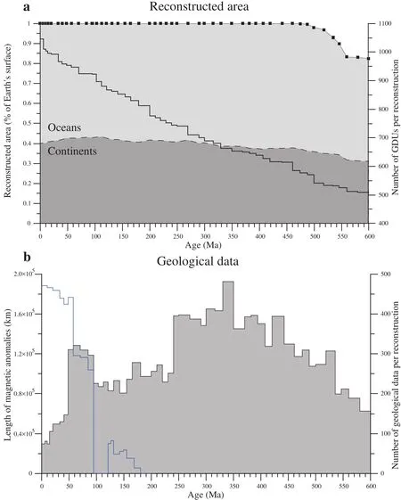
Figure 6 a-Evolution of the reconstructed area through time. Black squares represent the 48 reconstructions. Dashed line marks the limit between continental and oceanic area on each reconstruction. Black line represents the number of GDUs per reconstruction;b-Number of geological data used for each reconstruction. The minimum value is 74 (0 Ma), the maximum is 481 (330 Ma) and the average value is 267.4±101.0 (1σ) data per reconstruction. Blue line represents the length of measured isochrones available for each reconstruction after Müller et al. (2008a).

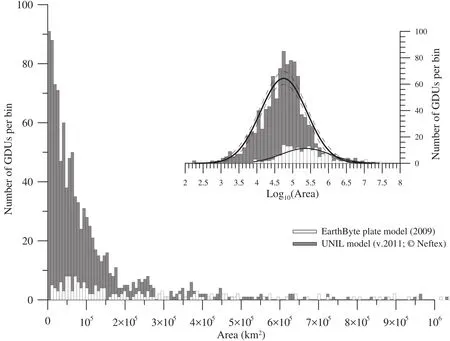
Figure 7 GDU size distribution. Number of GDUs per bins of 7500 km2. The minimum size is 0.183×103 km2 large and the maxi?mum is 1.65×107 km2 large. The distribution is logarithmically Gaussian and the mean value in log is of 4.74±0.65 corresponding to an area of 5.578×105 km2. The EarthByte plate model (2009; http://www.earthbyte.org/Resources/earthbyte_plate_model_2009.html)is shown for comparison. The number of blocks in their model (equivalent to our GDUs) is much inferior, and their mean size is much larger (2.334×106 km2).

The present model has been developed with ArcGIS?software. As all features making up the model are fully at?tributed (e.g., type, age), one can quantify various tectonic parameters anywhere on the globe and of any geological time, and thereafter develop a series of derivative maps(Figure 9b-9d). Using measured and synthetic isochrons,for example, we have computed palaeo?age maps repre?senting the age of the oceanic crust relative to the age of the reconstruction (see Figure 9b). Using Euler rotation poles describing plate motions, we calculate the veloci?ties and the convergence and divergence rates (Figure 9c;see also Vérardet al., 2012b). Moreover, following the approach of Turcotte and Schubert (2002), we are able to convert palaeo?ages into lithospheric thicknesses in order to estimate the volume of subducted materials (Figure 9d).

4 Discussion — Plate tectonic model and comparison with palaeoclimatic indicators

The model presented herein is based on years of field geology and thousands of literature studies. The output results are not strictly reproducible as input data are sub?jected to a degree of non?negligible interpretation. We do consider that temporal and spatial correlation of data reinforce their interpretation but one can always produce contradicting arguments that could deeply alter the model.Over the years, overhauls have occurred and some of our earliest publications are sometimes in contradiction with our latest version of the UNIL model (v.2011, ? Neftex).Many issues integrated in the model are still a matter of sharp debate and inherent assumptions cannot be detailed herein. The publication of GDU rotation poles, in particu?lar, would not be sufficient for other people to reproduce the model. Indeed, the redistribution of GDUs through space and time is only the first stage of the modeling pro?cess which must be followed by the redefinition of plate boundaries. Although strictly controlled by geological data, the latter step is in part subject to uncertainties and the ensuing result is proper to each author. Nevertheless, a first validation of our approach has been provided by the study of Hafkenscheidet al.(2006) which compared three tectonic models of Cenozoic-Mesozoic Tethyan evolu?tion with mantle tomography and concluded, as did Webb(2012), that our solution was the most reliable.

Figure 8 Plate size distribution throughout the Phanerozoic with linear scale in the foreground turned into log-log scale in the back?ground. The linear relationship (blue) with its associated 95% confidence interval (orange) in log-log scale shows the fractal behavior of plate size.

Here, we opt for a different but complementary ap?proach. We compare tectonic factors stemming from the reconstructions (2D maps on the globe) with separate pa?rameters such as palaeoclimatic indicators known to be strongly linked with plate tectonics. We are aware that processes involved in climate are nonlinear and complex.They concern, all at once, the bio?, hydro?, litho? and at?mosphere. They include positive and negative feedbacks which cannot be unveiled in a pure tectonic model. We,therefore, merely looked at first order (or large scale) cor?relations and did not expect to reproduce every single short scale variation.

4.1 Mean oceanic ages, plate velocities and sealevel variations

Using palaeo?age maps, we have calculated the aver?age age of the oceanic crust at each reconstruction (Fig?ure 10a). A noteworthy global negative trend can be ob?served. In the Early Cambrian (Fortunian), the oceanic crust is 16.8 million years old whereas, at present?day, the mean age is close to 65 million years old. The mathemati?

cal model (linear, logarithmic,etc.) behind this negative trend is unknown. However, a simple linear regression yields a secular decrease in mean oceanic age of -6.2%(coefficient of determination R2= 0.77, which is a classic statistical parameter). As the mean ocean ages, plate ve?locities (Figure 10b) also undergo a global decrease over the last 600 Ma (with a slope S equal to 0.0097 cm·yr-1/Ma). Although the coefficient of determination is low (R2= 0.36), the overall decrease is statistically confirmed at the 95% confidence level. We infer that the global aging of the lithosphere due to the overall slowdown of the plates is related to the reduction of the tectonic activity. The latter is potentially due to the global cooling of the Earth which has long been recognized (e.g., Kelvin, 1864; Turcotte, 1980;Labrosse and Jaupart, 2007) but never highlighted in a tec?tonic model. We note, furthermore, that when the linear trend (shown in Figure 10b) is extrapolated into the fu?ture, the line crosses the abscissa (i.e., mean plate motion equals zero cm·yr-1) at +500 Ma (and between +300 Ma and +1000 Ma at the 95% confidence level) suggesting the end of plate tectonics on Earth in this time frame (Figure 10d). Although one must be cautious with this because the decrease may well be nonlinear. One may think, therefore,that an evolution of Earth’s lithosphere similar to that of Mars might happen from then on.

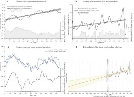
Figure 10 a-Mean palaeo?ages (i.e., relative to the age of the reconstruction) of oceanic floor over the Phanerozoic; the corresponding linear trendis shownwithits associated 95%confi?dence bounds. The grey step plot represents the standard deviation around the mean age at each reconstructed time slice andreflects the large dispersion around the mean value; b-Average velocities of plates for each reconstruction. Although the coefficient of determination is low(R2 =0.36), the overall decreasing trend is confirmed by the 95%confidence interval; c-Detrended oceanic mean age versus sea?level variations. Light blue, sea?level variations are from Haq et al. (1987) andHaq and Schutter (2008) (intermediate term); dark blue, sea?level variations are fromHaq et al. (1987) and Ross and Ross (1988). The blackcurve represents the detrended mean oceanic ages around its mean value (34.65 Ma; this study); d-Extrapolation of the linear trend displayed in b, showing that mean tectonic plate velocity reaches zero cm·yr-1 (i.e., stops) in ca. 500 Ma from now(dashed lines are 95%confidence limits) if the linear relationship is revealedto be true.

Possible causes for global sea?level changes are mul?tiple with various time?scales and amplitudes (see recent debate after the publication of Milleret al., 2005). On a long?term time scale (107yr to 108yr), sea-level fluctua?tions result from changes in the volume of ocean basins which are significantly, if not primarily, controlled by vari?ations of oceanic crust ages (e.g., Hays and Pitman, 1973;Parsons and Sclater, 1977; Donovan and Jones, 1979; Par?sons, 1982; Gaffin, 1987; Cognéet al., 2006; Cogné and Humler, 2008; Mülleret al., 2008b). Eustatic sea?level reconstructions based on stratigraphic data have been car?ried out by various authors (e.g., Vailet al., 1977; Hallam,1984; Haqet al., 1987; Haq and Schutter, 2008). Although Hallam (1984) shows a strong negative trend (-360 m)over the last 600 Ma, Vailet al.(1977) suggests a weak negative trend, and Haq and Schutter (2008) gives a posi?tive trend. A recent study by Parai and Mukhopadhyay(2012) further suggests that the global oceanic volume is near steady?state and that the observed trends are within the uncertainties. For comparison with the most recent study of Haq and Schutter (2008), we reduced the mean oceanic age from its secular trend (Figure 10c). At very first approximation, the resulting curve mimics the sealevel variation signal, especially for the last 450 Ma. Prior to 450 Ma, the mean age value is subject to caution as the reconstruction model does not cover the entire Earth sur?face. The possible absence of a global decreasing trend in the sea?level variation curve can be explained by the off?setting effect of plate deceleration. As the plates are mov?ing slower, the spreading rates are decreasing (Figure 11a;grey line). As a response, due to changes in the volume and composition of melt and to chemical variations in ba?salt composition (Klein and Langmuir, 1987; Keenet al.,1990; Bown and White, 1994; Humleret al., 1999), the in?itial ridge depth rises inducing a global uplift of the whole oceanic basement (see also Kominz, 1984; Stein and Stein,1992; Niu and Hekinian, 1997; Small and Danyushevsky,2003; Vérardet al., 2011, 2015). The main mismatch be?tween the sea level and the mean oceanic age curves ob?served around 170 Ma might result from the same process.The drop in mean oceanic age may be counterbalanced by a coeval velocity drop (Figure 11b) and is thought to have,therefore, no visible impact on the sea?level curve.

The parallel between palaeo?ages and sea?level varia?tions, even before 180 Ma, highlights the robustness of the reconstruction method for vanished oceans. The result is further confirmed by using a full topography (Vérardet al., 2015). However, we emphasize that the average value given here (i.e., the arithmetic mean) is not strictly statisti?cally representative as the surface/age distribution is not necessarily Gaussian distributed. Moreover, if predomi?nant, the mean age of the oceanic lithosphere is not the only driver of the eustatic sea?level change. Various pro?cesses, other than mid?oceanic ridge dynamics, can affect sea level over tens or hundreds of millions of years (e.g.,continental lithosphere variations, oceanic sediments vol?ume changes, ocean temperature variations, ocean volume variations,etc.).

4.2 Tectonic activity, carbon dioxide and glaciation

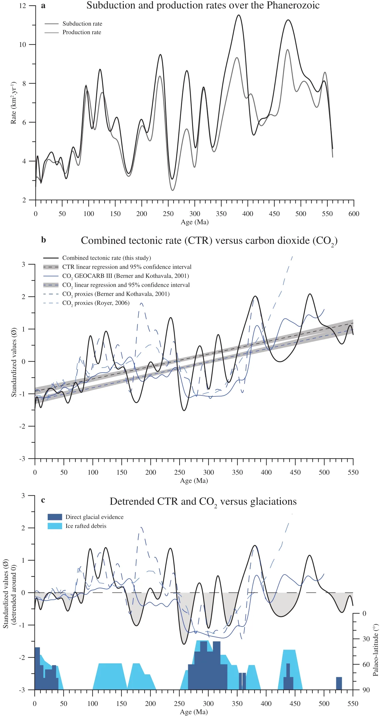
Figure 11 a-Evolution of subduction and production rates over the Phanerozoic. Subduction rates (black line) and production rates(grey line) are defined as the area of subducted/accreted material between two successive reconstructions; b-“Tectonic activity” (TA;black line) is the mean value between subduction and production rates. Linear decreasing trends of TA (R2 = 0.44) and CO2 (R2 = 0.49)are confirmed by 95% confidence intervals. The slopes are very similar (STA = 0.00394 and SCO2 = 0.00399); c-Direct glacial evidence(tillites, striated bedrock, etc.; dark blue) are from Royer et al. (2004) modified after Crowley and Burke (1998). Ice rafted debris (light blue) are from Frakes and Francis (1988).

When analyzing the relationship between the area of preserved oceanic lithosphere per unit time versus age,Parsons (1982) and later Rowley (2002) observed a lin?ear decrease in the area of ocean age with increasing age.Such a linear trend is contrary to what one would expect if oceanic accretion rates varied significantly through time.As an explanation, the authors raised the hypothesis of a constant destruction (and therefore production) rate of the oceanic crust through time. However, a long term steady?state production rate is unlikely for, at least, three reasons:(1) the present-day spreading rates vary significantly from ocean to ocean (from 0.73 cm·yr-1in the Arctic Ocean to 18 cm·yr-1in the Pacific Ocean; DeMetset al., 1990); (2)spreading rates calculated thanks to preserved magnetic anomalies have strongly varied since Jurassic times (Kom?inz, 1984; Larson, 1991; Mülleret al., 2008a). In Gaffin’s(1987) model, for instance, the production rates in the Cretaceous are almost double relative to present?day; (3)tectonic processes such as ridge jump, ridge subduction,back?arc opening, continental breakup and continental col?lision are frequent and result in abrupt changes in plate motions. Moreover, Demicco (2004) showed that it was possible to achieve the same linear relationship as in Par?sons (1982), even accounting for non?steady?state produc?tion of oceanic crust with time. Figure 11a represents the subduction and production rates (in km2·yr-1) stemming from the UNIL model (v.2011, ? Neftex; defined as the area of subducted/produced material divided by the length of trenches/ridges respectively). For the Cretaceous, the results are in good agreement with the studies of Gaffin(1987), Larson (1991), Mülleret al.(2008b) on production rates and Engebretsonet al.(1992) on subduction rates,but in contradiction with that of Cogné and Humler (2006),presenting slightly lower rates. Over the Phanerozoic, we can observe that production rates have strongly varied be?tween a minimum of 2.48 km2·yr-1and a maximum of 9.74 km2·yr-1which is contradictory to the steady?state model.

Although, in Figure 11a, the production and subduction rates are closely related, the two curves present local dis?crepancies due to intra?plate deformations (i.e., extension in rifting and shortening in collision zones). We thus in?troduce a “tectonic activity” (TA) parameter representing the average value between production and subduction rates and reflecting the global tectonic activity of the Earth. In order to compare parameters having different units, the val?ues are standardized using the following equation (eq. 1):

where, μ is the mean and σ is the standard deviation of the dataset.

Global plate motion changes have a predominant effect on long term variations of carbon dioxide (e.g., Berneret al., 1983; Lasagaet al., 1985). During orogenies, the weathering of silicate rocks removes carbon from the at?mosphere (by fixing it as additional carbonate;e.g., Urey,1952). The return of this carbon to the atmosphere via met?amorphism, diagenesis and volcanism may take hundreds of millions of years. Such delay can result in an imbal?ance in CO2exchanges between atmosphere and rock res?ervoirs. Carbon dioxide variations are thus closely linked to the rate of sea-floor generation and subduction. We note that models developed to simulate the Phanerozoic evolu?tion of atmospheric CO2composition (Berner and Kothav?ala, 2001; Wallmann, 2004; Berner, 2006) use weathering and degassing variations due to tectonics as key input pa?rameters.

Our data are compared with the GEOCARB III CO2model of Berner and Kothavala (2001) associated with the proxy data of Berner and Kothavala (2001) and Roy?er (2006) based on palaeosols, stomata, phytoplankton,boron and liverworts analyses (Figure 11b). At the first order, the records have some good parallels. As expect?ed (following palaeo?ages and plate velocities), the TA undergoes a global decrease over the Phanerozoic. The trend is indeed remarkably similar with the overall down?ward trend of the CO2curve (slopes are STA= 0.00394 and SCO2= 0.00399), highlighting the link between CO2and tectonics. In details, short term fluctuations (10 Ma to 20 Ma) observed in the TA signal are rarely reflected in the GEOCARB III model whereas they are sometimes observed in the proxies. Albeit not statistically signifi?cant, the agreement is better on the larger scale. From the Cambrian to the Silurian (600 Ma to 400 Ma), high levels of CO2correspond to high levels of TA. In the same way,the CO2drop extending from the Early Devonian to the Early Permian (380-280 Ma) is coeval with a lowering of TA. Last, from 150 Ma to the present, the global decrease of the CO2coincides with a reduction of TA. The secular decreasing trend of CO2has long been recognized. An ex?planation is given by Berner (2004) who showed that the negative slope of the CO2curve is flattened when holding the solar luminosity constant over the time. Conversely, a slow increase in the luminosity of the sun causes warm?ing, faster weathering and consequent CO2removal from the atmosphere to be fixed ultimately as carbonates. One of the major features noticeable both in the GEOCARB III model and in proxy estimates is the very low level of CO2observed during the Permo?Carboniferous. After Berner (1998), a primary reason for this drop was the rise of large vascular land plants, which accelerated weather?ing and led to the burial of large quantities of organic matter in sediments. Here, we can see that, coeval with the emergence of large vascular plants, a strong decrease of tectonic activity occurred. The two processes likely acted in the same direction.

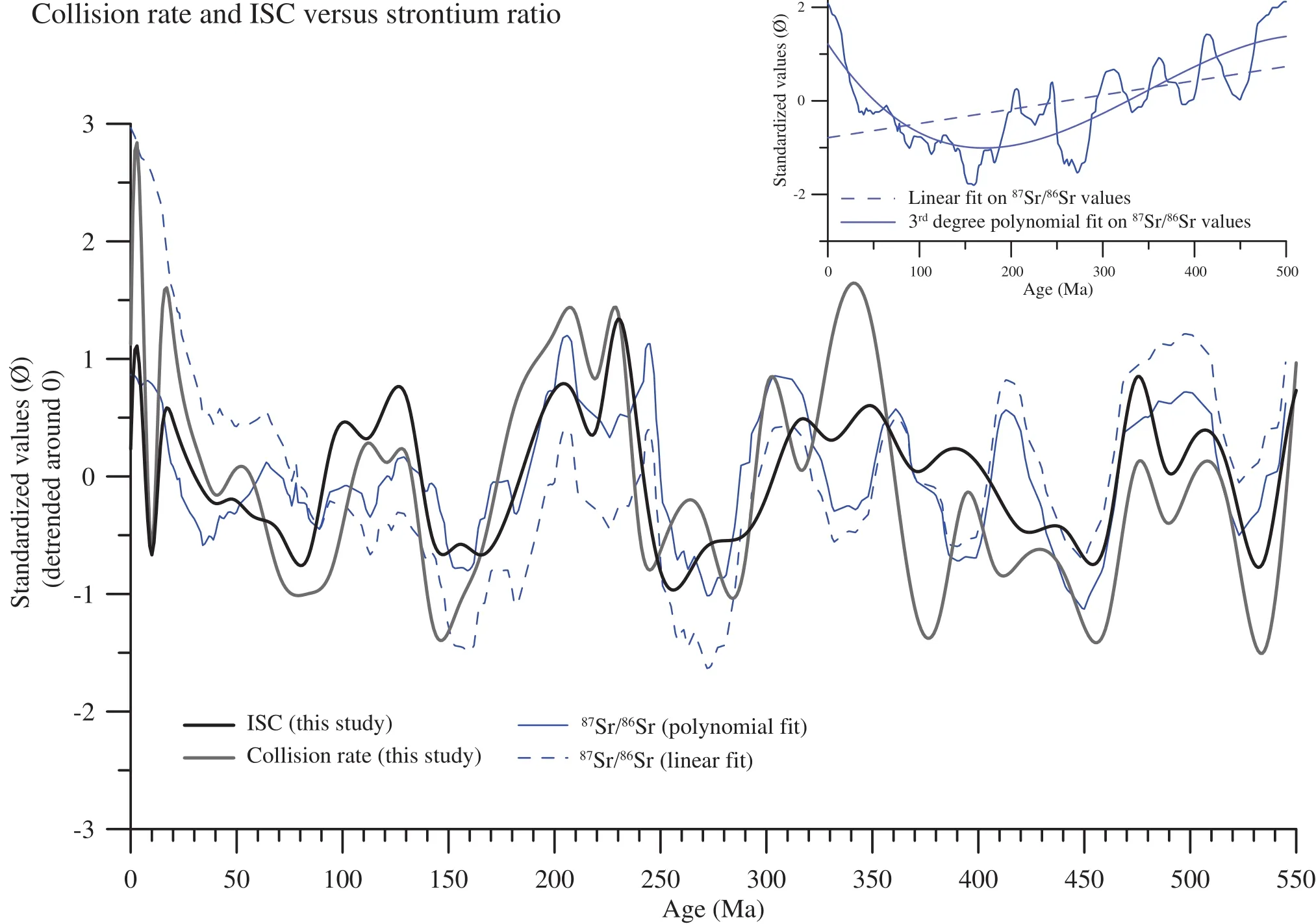
Figure 12 Comparison between reduced (or detrended) curves: “impact strontium curve” (ISC — black line; see text), collision rates (grey line) and strontium ratio (blue lines). Inset: 87Sr/86Sr ratio after Prokoph et al. (2008) showing the two fits used for data reduction.

Carbon dioxide is thought to be the primary impacting factor on climate (Royeret al., 2004). Latitudinal exten?sion of glaciation evidence (Frakes and Francis, 1988;Frakeset al., 1992; and modified from Crowley and Burke,1998 in Royeret al., 2004) is thus compared with tectonic activity and CO2curves, detrended from their secular de?crease (Figure 11c). The “tectonic activity” (TA) curve is in good agreement with the glaciation records. Not only do the long?lived Paleozoic and Cenozoic glaciations show up as relatively negative values in the detrended TA curve(Figure 11c), but also the shorter and sometimes less firm?ly identified Early Cambrian (Crowley and Burke, 1998),Late Ordovician (e.g., Saltzman and Young, 2005; Cherns and Wheeley, 2007) and Late Jurassic ones (e.g., Dromartet al., 2003; Suanet al., 2010). Only the short?lived Late Devonian to Early Carboniferous glaciation (e.g., Dickins,1993) is not detectable with the model, which is visible in the CO2records. The existence of a relatively cool period between the Middle Jurassic and the Early Cretaceous, if it exists (Alley and Frakes, 2003), is neither supported by the CO2model and proxies nor by the tectonic model (UNIL model, v.2011, ? Neftex).

4.3 Collision zones and strontium ratio

Strontium data are probably the most reliable isotop?ic record available for the whole Phanerozoic. Since no strontium isotopic fractionation occurs during carbonate precipitation and deposition, isotopic ratios measured from carbonates reflect that of seawater (Francois and Walker,1992). The current strontium composition of seawater is a balance between inputs of high87Sr/86Sr (ca. 0.715) due to the weathering of continental igneous rocks and low87Sr/86Sr (ca. 0.703) resulting from fluid exchanges in sea?floor hydrothermal systems. The 0.715 Sr-value for conti?nental rocks is a weighted average between the presently exposed87Sr?enriched (ca. 0.718) old shields and87Sr?de?pleted (ca. 0.705) young igneous rocks, which is close to the oceanic Sr?ratio (ca. 0.709; Francois and Walker, 1992 and references therein). Therefore, the oceanic Sr?ratio can be presumed as a balance between the accretion of new oceanic crust and the exposure and weathering of old igne?ous rocks during collisions. In most box models developed to simulate the Phanerozoic seawater composition, the Sr?ratio of oceans is used as a proxy of mountain building(seee.g., Berner, 1994, 2006; Wallmann, 2001).

For comparison purposes, we computed an “impact strontium curve” (ISC) (Figure 12) representing the av?erage between the standardized values of production and collision rates. Note that, in the UNIL model (v.2011; ?Neftex), a distinction is made between active collision zones (i.e., converging plate boundaries) and suture zones(inactive collision zones located inside plates). The col?lision rate is defined as the overlapped area between two plates during a collision divided by the length of the colli?sion zone. Although suture zones (i.e., old and mostly in?active collision zones) also correspond to mountain belts,they are not taken into account in the ISC calculation (see Vérardet al., 2015 for alternate calculation). Another bias could also stem from the lack of consideration of the rock age involved in the collision since young and old igne?ous rocks have opposite87Sr/86Sr values. Last, ISC does not account for spatial distributions of collision zones and precipitations which might be of major concern (Tardyet al., 1989). Newly created mountain belts, indeed, have no impact on87Sr/86Sr ratio if they are not subject to erosion.

Using a comprehensive database of low?Mg calcitic fossil shells, Prokophet al.(2008) demonstrated that among87Sr/86Sr, δ34S, δ18O and δ13C isotopes, the δ18O re?cord was the only record with a significant linear trend through the Phanerozoic. However, Veizeret al.(1999)established a strong correlation between the87Sr/86Sr and the δ18O signals which implies that strontium ratio should undergo a similar decrease over the Phanerozoic. As a consequence, in order to compare with the ISC, we have detrended the87Sr/86Sr curve, once with a linear fit (with a poor R2value of 0.21) and once with a third degree polynomial fit (with a better R2value of 0.68). Whatever the method chosen, the UNIL model (v.2011, ? Neftex)follows a good agreement with the detrended87Sr/86Sr variations (Figure 12). Except during the Devonian-Car?boniferous times, the ISC reproduces correctly most of the main Sr?ratio maxima and minima. Three causes may be invoked for the remaining local temporal shifts (par?ticularly between 450 Ma and 350 Ma): (1) errors in the geodynamical model cannot be ruled out, and the model should therefore be revised if incorrect; (2) as the ISC results from a simple arithmetic mean, no consideration is given to the relative weights of old versus young igne?ous rocks and hydrothermal flux versus weathering flux;(3) the lack of temporal integration in the calculation of instantaneous production and collision rates. However,even if the ISC calculation seems relatively crude in comparison to the complexity of the strontium cycle, the correlation between the two curves is better than when one only considers the collision rates (grey curve on Fig?ure 12). This underlines again the robustness of the re?construction approach for vanished oceans.

5 Conclusions

We have developed the first global and physically co?herent geodynamic model covering the entire Earth's sur?face for the whole Phanerozoic. For the first time, (1) a long term decrease of plate velocities (together with an ag?ing of the oceanic crust, as expected) is observed in a set of global reconstructions; (2) we have been able to quan?tify oceanic production rates over the past 600 Ma and the results support the idea of a non?steady?state production of oceanic crust with time. We speculate that the overall decrease of tectonic activity is a consequence of global cooling of the Earth system.

In their study, Veizeret al.(1999) established a strong correlation between87Sr/86Sr, δ18O and δ13C variations over the Phanerozoic at any resolution greater than 1 Ma. With?out further evidence, the authors state that this correlation suggests that the exogenic system (defined as litho-, hy?dro?, atmo?, and biosphere) was strongly driven by tec?tonic forces. All calculations shown herein are based on 2D spherical maps. More direct comparison of sea?level changes and strontium fluctuations is studied using an in?novative 3D conversion (full topography) of the present model (Vérardet al., 2015). Nevertheless, the first order correlation between the tectonic factors (i.e., plate veloci?ties, mean oceanic ages, accretion, subduction and colli?sion rates) stemming from the UNIL model (v.2011; ?Neftex) with a combination of palaeoclimatic indicators(i.e., Sr?ratio, atmospheric carbon dioxide, sea?level varia?tions and glacial deposits) supports the idea that plate tec?tonics has a predominant effect on climate at a scale of 107yr-1to 108yr-1.

Acknowledgements

We gratefully thank all members of the Prof. Stampfli’s working group for sharing their data, ideas, and time with us. The Institute of Geology and Palaeontology of the Uni?versity of Lausanne (UNIL) and the Swiss National Fund(SNF) are equally acknowledged for funding the present work. We thank Dr. Karin Warners?Ruckstuhl and Dr.Xiu?Mian Hu, for their comments and suggestions. The geodynamic model is now the property of Neftex Petro?leum Consultants Ltd., with license to UNIL. We grate?fully acknowledge the permission from Neftex Petroleum Consultants Ltd. to publish these results.