Diffusion models for time-series applications:a survey

Lequan LIN, Zhengkun LI, Ruikun LI, Xuliang LI, Junbin GAO

1Discipline of Business Analytics, The University of Sydney Business School, Camperdown, NSW 2006, Australia

2Postdoctoral Programme of Zhongtai Securities Co., Ltd., Jinan 250000, China

E-mail: lequan.lin@sydney.edu.au; lizk@zts.com.cn; ruikun.li@sydney.edu.au;xuli3128@uni.sydney.edu.au; junbin.gao@sydney.edu.au

Received Apr.29, 2023; Revision accepted Sept.18, 2023; Crosschecked Nov.28, 2023; Published online Dec.28, 2023

Abstract: Diffusion models, a family of generative models based on deep learning, have become increasingly prominent in cutting-edge machine learning research.With distinguished performance in generating samples that resemble the observed data, diffusion models are widely used in image, video, and text synthesis nowadays.In recent years, the concept of diffusion has been extended to time-series applications, and many powerful models have been developed.Considering the deficiency of a methodical summary and discourse on these models, we provide this survey as an elementary resource for new researchers in this area and to provide inspiration to motivate future research.For better understanding, we include an introduction about the basics of diffusion models.Except for this, we primarily focus on diffusion-based methods for time-series forecasting, imputation, and generation, and present them, separately, in three individual sections.We also compare different methods for the same application and highlight their connections if applicable.Finally, we conclude with the common limitation of diffusion-based methods and highlight potential future research directions.

Key words: Diffusion models; Time-series forecasting; Time-series imputation; Denoising diffusion probabilistic models; Score-based generative models; Stochastic differential equations

1 Introduction

Diffusion models, a family of deep-learningbased generative models, have risen to prominence in the machine learning community in recent years(Croitoru et al., 2023; Yang L et al., 2023).With exceptional performance in various real-world applications such as image synthesis (Austin et al., 2021;Dhariwal and Nichol, 2021; Ho et al., 2022a), video generation (Harvey et al., 2022; Ho et al., 2022b;Yang RH et al., 2022), natural language processing(Li XL et al., 2022; Nikolay et al., 2022; Yu et al.,2022),and time-series prediction(Rasul et al.,2021;Li Y et al.,2022;Alcaraz and Strodthoff, 2023),diffusion models have demonstrated their power over many existing generative techniques.

Given some observed dataxfrom a target distributionq(x),the objective of a generative model is to learn a generative process that produces new samples fromq(x)(Luo C,2022).To learn such a generative process,most diffusion models begin by progressively disturbing the observed data by injecting Gaussian noise, and then applying a reversed process with a learnable transition kernel to recover the data(Sohl-Dickstein et al., 2015;Ho et al., 2020;Luo C, 2022).Typical diffusion models assume that after a certain number of noise injection steps, the observed data will become standard Gaussian noise.So, if we can find the probabilistic process that recovers the original data from standard Gaussian noise,then we can generate similar samples using the same probabilistic process with any random standard Gaussian noise as the starting point.

The recent three years have witnessed the extension of diffusion models to time-series-related applications, including time-series forecasting (Rasul et al., 2021; Li Y et al., 2022;Bilo? et al., 2023),time-series imputation(Tashiro et al.,2021;Alcaraz and Strodthoff,2023;Liu MZ et al.,2023),and timeseries generation(Lim et al., 2023).Given observed historical time series, we often try to predict future time series.This process is known as time-series forecasting.Because observed time series are sometimes incomplete due to reasons such as data collection failures and human errors, time-series imputation is implemented to fill in the missing values.Different from time-series forecasting and imputation,time-series generation or synthesis aims to produce more time-series samples with characteristics similar to the observed period.

Basically, diffusion-based methods for timeseries applications are developed from three fundamental formulations, including denoising diffusion probabilistic models (DDPMs), score-based generative models(SGMs),and stochastic differential equations (SDEs).The target distributions learned by the diffusion components in different methods often involve the condition on previous time steps.Nevertheless,the design of the diffusion and denoising processes varies with different task objectives.Hence, a comprehensive and self-contained summary of relevant literature will be an inspiring beacon for new researchers who are just entering this new-born area and experienced researchers who seek future directions.Accordingly, this survey aims to summarize the literature, compare different approaches, and identify potential limitations.

In this paper, we review diffusion-based models for time-series applications (refer to Table 1 for a quick summary).For better understanding, we include a brief introduction about three predominant formulations of diffusion models in Section 2.Next,we categorize the existing models based on their major functions.Specifically, we discuss the models primarily for time-series forecasting, time-series imputation, and time-series generation in Sections 3,4, and 5, respectively.In each section, we have a separate subsection for problem formulation, which helps clarify the objective, training, and forecasting settings of each specific application.We highlight if a model can serve multiple purposes and articulate the linkage when one model is related to or slightly different from another.In Section 6,we compare all the models mentioned in this review on some specific aspects such as their diffusion formulation and sampling processes.In Section 7, we briefly introduce some practical application domains in the real world while providing good sources of publicly available datasets.Furthermore,we discuss some current limitations and challenges faced by researchers and practitioners to inspire future research in Section 8.Eventually,we conclude this survey in Section 9.

2 Basics of diffusion models

The underlying principle of diffusion models is to progressively perturb the observed data with a forward diffusion process and then recover the original data through a backward reverse process.The forward process involves multiple steps of noise injection,where the noise level changes at each step.The backward process, in contrast, consists of multiple denoising steps that aim to remove the injected noise gradually.Normally,the backward process is parameterized by a neural network.Once the backward process has been learned, it can generate new samples from almost arbitrary initial data.Stemming from this basic idea, diffusion models are predominantly formulated in three ways: DDPMs, SGMs,and SDEs.

In this section, we discuss the theoretical background of diffusion models before introducing the above-mentioned formulations.By doing this, we aim to lead readers who are not deeply familiar with this area from traditional generative concepts to diffusion models.

2.1 Background of diffusion models

Generative models are designed to generate samples from the same distribution of the observed dataxby learning the approximation of the true distributionq(x).To achieve this, many methods assume that the observed data can be generated from some invisible data or the so-called latent variable.The learning task then becomes minimizing the variational lower bound of the negative log-likelihood of the target distribution with some learnable parameters associated with the distribution of the latent variable.Variational autoencoder (VAE) is one of the most widely known methods built on this assumption (Kingma and Welling, 2013).While the VAE is based on a single latent variable, the hierarchical variational autoencoder(HVAE)generalizesthe idea to multiple latent variables with hierarchies,enhancing the flexibility of the underlying generative assumptions (Kingma et al., 2016; S?nderby et al.,2016).

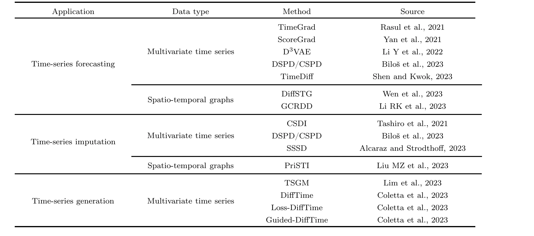
Table 1 A summary of diffusion-based methods for time-series applications

Diffusion models were originally introduced in Sohl-Dickstein et al.(2015).Then some improvements proposed by Ho et al.(2020)endowed diffusion models with remarkable practical value, contributing to their conspicuous popularity nowadays.As a matter of fact, diffusion models can be seen as an extension of the HVAE, constrained by the following restrictions: (1) the latent variables are under a Markov assumption, effectively leading to a Markov chain based generative process;(2)the observed data and latent variables share the same dimension; (3)the Markov chain is linked by Gaussian transition kernels, and the last latent variable of the chain is from the standard Gaussian distribution.For better understanding,we illustrate the connections and differences between traditional generative models and diffusion models in Fig.1.

2.2 Denoising diffusion probabilistic models

DDPMs implement the forward and backward processes through two Markov chains (Sohl-Dickstein et al., 2015;Ho et al.,2020).Let the original observed data bex0, where 0 indicates that the data are free from the noises injected in the diffusion process.

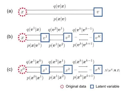
Fig.1 Comparison of traditional generative models and the diffusion model: (a) variational autoencoder;(b) Markov hierarchical variational autoencoder; (c)diffusion model

The forward Markov chain transformsx0to a sequence of disturbed datax1,x2,...,xKwith a diffusion transition kernel:

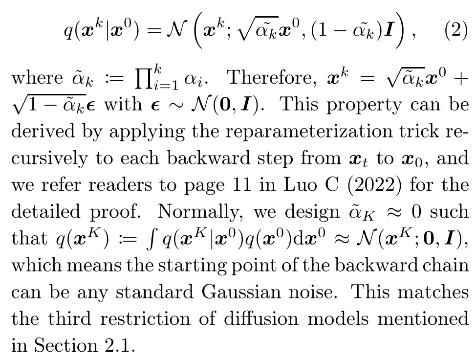
whereαk ∈(0,1)fork=1,2,...,Kare hyperparameters indicating the changing variance of the noise level at each step,andN(x;μ,Σ)is the general notation for the Gaussian distribution ofxwith the meanμand the covarianceΣ.A nice property of this Gaussian transition kernel is that we may obtainxkdirectly fromx0by

Assuming that the backward process can also be realized with a Gaussian transition kernel,the reverse transition kernel is modeled by a parameterized neural network:

whereθdenotes learnable parameters.Now, the remaining problem is how to estimateθ.Basically,the objective is to maximize the likelihood objective function so that the probability of observing the training samplex0estimated bypθ(x0)is maximized.This task is accomplished by minimizing the variational lower bound of the estimated negative log-likelihood-logq(x0),that is,

wherex0:Kdenotes the sequencex0,x1,...,xK.

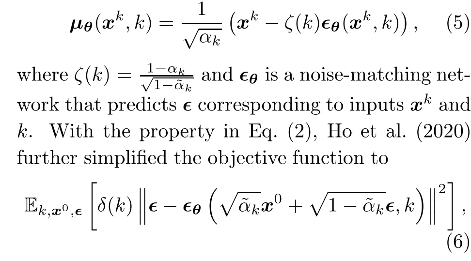
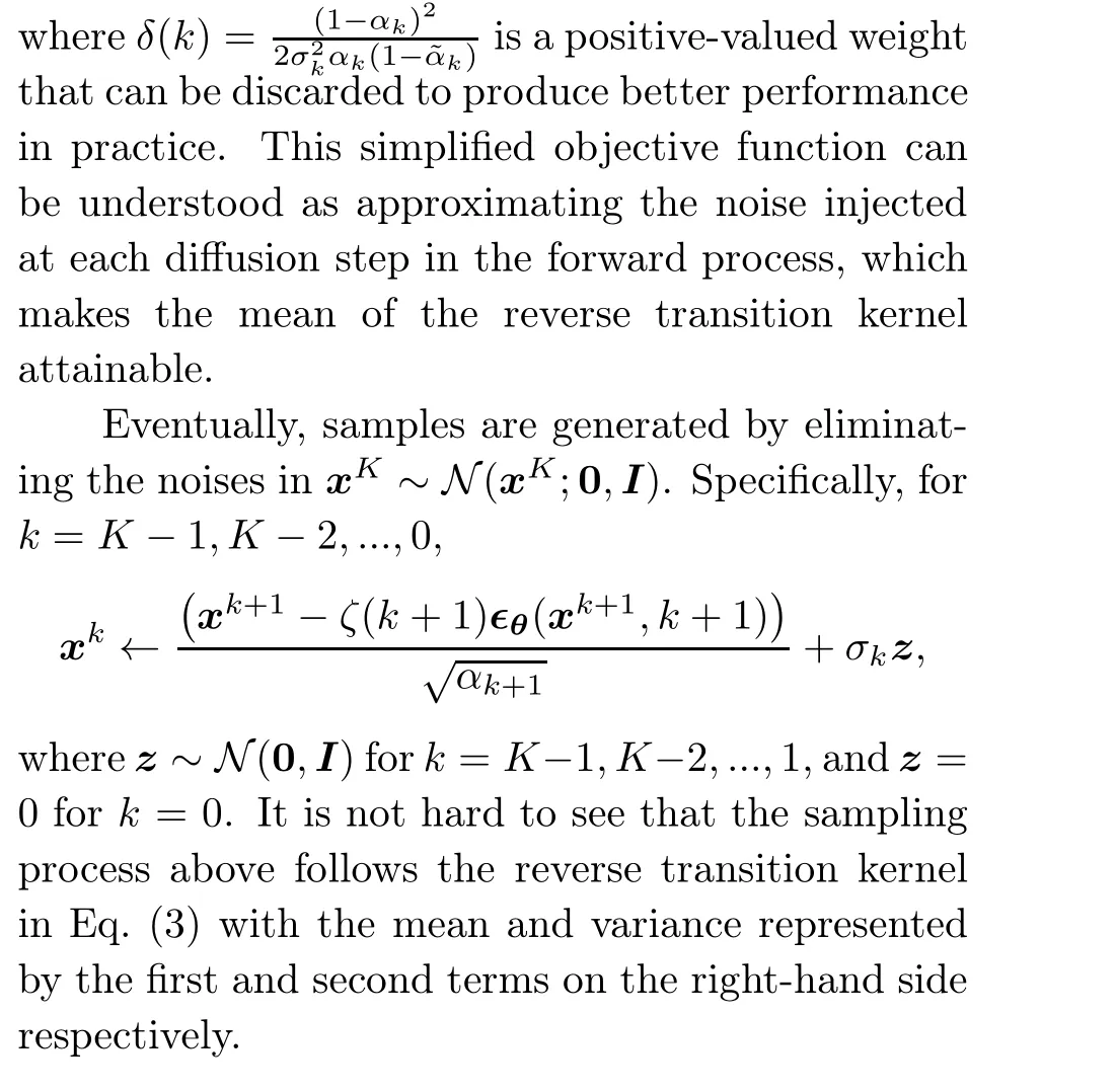
Ho et al.(2020) proposed that we could simplify the covariance matrixΣθ(xk,k) in Eq.(3) as a constant-dependent matrixσ2kI,whereσ2kcontrols the noise level and may vary at different diffusion steps.In addition, they rewrote the mean as a function of a learnable noise term as

2.3 Score-based generative models

SGMs consist of two modules, including score matching and annealed Langevin dynamics (ALD).ALD is a sampling algorithm that generates samples with an iterative process by applying Langevin Monte Carlo at each update step (Song Y and Ermon,2019).Stein score is an essential component of ALD.The Stein score of a density functionq(x) is defined as?xlogq(x), which can be understood as a vector field pointing in the direction in which the log-likelihood of the target distribution grows most quickly.Because the true probabilistic distributionq(x) is usually unknown, score matching (Hyv?rinen, 2005)is implemented to approximate the Stein score with a score-matching network.Here we primarily focus on denoising score matching (Vincent,2011) because it is empirically more efficient, but other methods such as sliced score matching (Song Y et al., 2020) are also commonly mentioned in the literature.

The underlying principle of denoising score matching is to process the observed data with the forward transition kernelq(xk|x0) =N(xk;x0,σ2kI),withσ2kbeing a set of increasing noise levels fork= 1,2,...,K, and then to jointly estimate the Stein scores for the noise density distributionsqσ1(x),qσ2(x),...,qσk(x)(Song Y and Ermon,2019).The Stein score for noise density functionqσk(x) is defined as?xlogqσk(x).Once the Stein scores are found,samples can be generated with ALD by gradually pushing random white noises towards highdensity regions of the target distribution along the direction pointed by these scores.

Usually, the Stein score is approximated by a neural networksθ(x,σk), whereθcontains learnable parameters.Accordingly, the initial objective function is given as

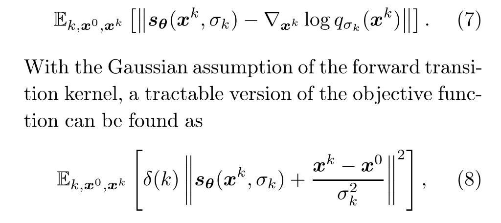
whereδ(k) is a positive-valued weight depending on the noise scaleσk.

After the score-matching networksθis learned,the ALD algorithm will be implemented for sampling.The algorithm is initialized with a sequence of increasing noise levelsσ1,σ2,...,σKand a starting pointxK,0～N(0,I).Fork=K,K-1,...,0,xkwill be updated withNiterations that compute

wheren=1,2,...,N,z～N(0,I),andηkrepresents the update step.Note that after eachNiterations,the last outputxk,Nwill be assigned as the starting point of the nextNiterations, that is,xk-1,1.x0,Nwill be the final sample.The role ofzin this sampling process is to add slight uncertainty, such that the algorithm will not end up with almost identical samples.

2.4 Stochastic differential equations

DDPMs and SGMs implement the forward pass as a discrete process, which means we should carefully design the diffusion steps.To overcome this limitation,one may consider the diffusion process as continuous such that it becomes the solution of an SDE (Yang S et al., 2021).This formulation can be thought of as a generalization of the previous two formulations, because both DDPMs and SGMs are discrete forms of SDEs.The backward process is modeled as a time-reverse SDE, and samples can be generated by solving this time-reverse SDE.Letwand ?wbe a standard Wiener process and its timereverse version, respectively, and consider a continuous diffusion timek ∈[0,K].A general expression of SDE is

and the time-reverse SDE, as shown by Anderson(1982),is

In addition,Yang S et al.(2021)illustrated that sampling from the probability flow ordinary differential equation(ODE)as follows has the same distribution as the time-reverse SDE:

Heref(x,k) andg(k) separately compute the drift coefficient and the diffusion coefficient for the diffusion process.?xlogqk(x) is the Stein score corresponding to the marginal distribution ofxk,which is unknown but can be learned with a similar method as in SGMs with the objective function

Therefore,the training objective is once again to find a neural networksθ(xk,k)to approximate the Stein scores.However, because the Stein scores here are instead based on a continuous process, the subtraction term cannot be simplified as before, and the SDE of the diffusion process is required before one can derive the Stein scores for approximation.

Now, how to write the diffusion processes of DDPMs and SGMs as SDEs? Recall thatαkis a defined parameter in DDPMs and thatσ2kdenotes the noise level in SGMs.The SDE corresponding to DDPMs is known as a variance preserving (VP)SDE, and is defined as

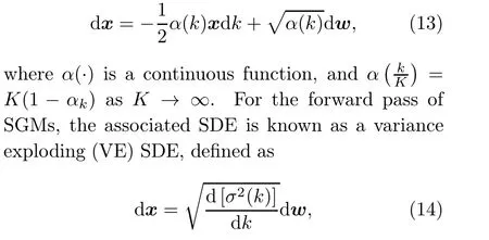
whereσ(·) is a continuous function, andσ(kK) =σkasK →∞(Yang S et al., 2021).Inspired by the VP SDE,Yang S et al.(2021)designed another SDE called the sub-VP SDE, which performs especially well on likelihoods, and is given by

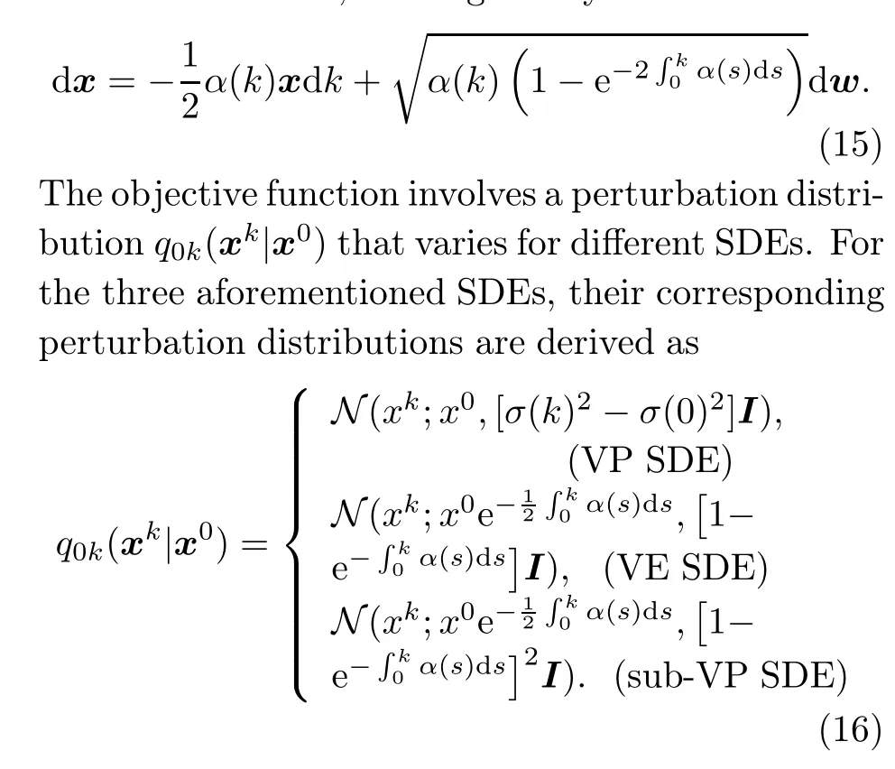
After successfully learningsθ(x,k),samples are produced by deriving the solutions to the time-reverse SDE or the probability flow ODE with techniques such as ALD.

3 Time-series forecasting

Multivariate time-series forecasting is a crucial area of study in machine learning research, with wide-ranging applications across a variety of industries.Different from the univariate time series,which tracks only one feature over time, the multivariate time series involves the historical observations of multiple features that interact with each other and evolve with time (Fig.2).Consequently, multivariate time series provide a more comprehensive understanding of complex systems and realize more reliable predictions of future trends and behaviours.

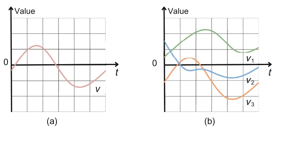
Fig.2 Examples of a univariate time series (a) and a multivariate time series (b)

In recent years, generative models have been implemented for multivariate time-series forecasting tasks.For example, WaveNet is a generative model with dilated causal convolutions that encode longterm dependencies for sequence prediction (van den Oord et al.,2016).As another example,Kashif et al.(2021) modeled a multivariate time series with an autoregressive deep learning model, in which the data distribution is expressed by a conditional normalizing flow.Nevertheless, the common shortcoming of these models is that the functional structure of their target distributions is strictly constrained.Diffusion-based methods, on the other hand, can provide a less restrictive solution.In this section,we will discuss five diffusion-based approaches.We also discuss two models designed specifically for spatiotemporal graphs (i.e., spatially related entities with multivariate time series) to highlight the extension of diffusion theories to more complicated problem settings.Because relevant literature mostly focuses on multivariate time-series forecasting,“forecasting”refers to multivariate time-series forecasting in the rest of this survey unless otherwise stated.

3.1 Problem formulation

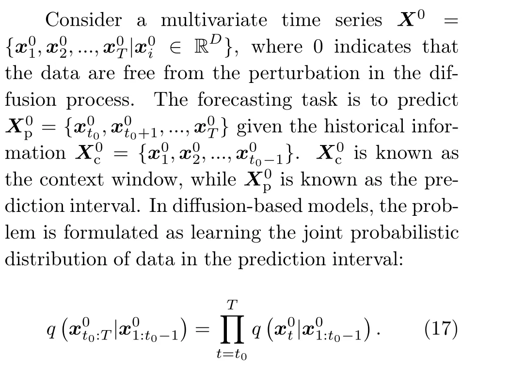
Some literature also considers the role of covariates in forecasting, such as Rasul et al.(2021)and Yan et al.(2021).Covariates are additional information that may impact the behavior of variables over time, such as seasonal fluctuations and weather changes.Incorporating covariates in forecasting often helps strengthen the identification of factors that drive temporal trends and patterns in data.The forecasting problem with covariates is formulated as

wherec1:Tdenotes the covariates for all time points and is assumed to be known for the whole period.

For the purpose of training, one may randomly sample the context window followed by the prediction window from the complete training data.This process can be seen as applying a moving window with sizeTon the whole timeline.Then, the optimization of the objective function can be conducted with the samples.Forecasting a future time series is usually achieved by the generation process corresponding to the diffusion models.

3.2 TimeGrad

The first noticeable work on diffusion-based forecasting is TimeGrad proposed by Rasul et al.(2021).Developed from DDPMs, TimeGrad first injects noise to data at each predictive time point,and then gradually denoises through a backward transition kernel conditioned on historical time series.To encode historical information,TimeGrad approximates the conditional distribution in Eq.(18)by

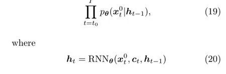
is the hidden state calculated with a recurrent neural network (RNN) module such as long shortterm memory (LSTM) (Hochreiter and Schmidhuber, 1997) or gated recurrent unit (GRU) (Chung et al., 2014) that can preserve historical temporal information, andθcontains learnable parameters for the overall conditional distribution and its RNN component.

The objective function of TimeGrad is in the form of a negative log-likelihood,given as

where for eacht ∈[t0,T],-logpθ(x|ht-1)is upper bounded by

The context window is used to generate the hidden stateht0-1for the starting point of the training process.It is not hard to see that Eq.(22) is very similar to Eq.(6) except for the inclusion of hidden states to represent the historical information.

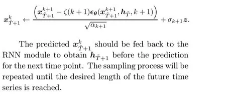
In the training process, the parameterθis estimated by minimizing the negative log-likelihood objective function with stochastic sampling.Then,future time series are generated in a step-by-step manner.Suppose that the last time point of the complete time series is ?T.The first step is to derive the hidden stateh?Tbased on the last available context window.Next, the observation for the next time point ?T+1 is predicted in a manner similar to DDPMs:

3.3 ScoreGrad

ScoreGrad shares the same target distribution as TimeGrad,but it is alternatively built upon SDEs,extending the diffusion process from discrete to continuous and replacing the number of diffusion steps with an interval of integration (Yan et al., 2021).ScoreGrad is composed of a feature extraction module and a conditional SDE-based score-matching module.The feature extraction module is almost identical to the computation ofhtin TimeGrad.However, Yan et al.(2021) discussed the potential of adopting other network structures to encode historical information, such as temporal convolutional networks(van den Oord et al., 2016)and attentionbased networks(Vaswani et al.,2017).Here,we still focus on RNN as the default choice.In the conditional SDE-based score-matching module, the diffusion process is conducted through the same SDE as in Eq.(9) but its associated time-reverse SDE is refined as

wherek ∈[0,K] represents the SDE integral time.As a common practice, the conditional score function?xtlogqk(xt|ht) is approximated with a parameterized neural networksθ(xkt,ht,k).Inspired by WaveNet (van den Oord et al., 2016) and Diff-Wave (Kong et al., 2021), the neural network is designed to have eight connected residual blocks,while each block contains a bidirectional dilated convolution module, a gated activation unit, a skipconnection process, and a one-dimension (1D) convolutional neural network for output.

The objective function of ScoreGrad is a conditional modification of Eq.(12),computed as

Up to this point,we use only the general expression of SDE for simple illustration.In the training process, one shall decide the specific type of SDE to use.Potential options include VE SDE, VP SDE,and sub-VP SDE (Yang S et al., 2021).The optimization varies depending on the chosen SDE, because different SDEs lead to different forward transition kernelsq(xkt|xk-1t) and also different perturbation distributionsq0k(xt|x0t).Finally, for forecasting, ScoreGrad uses the predictor-corrector sampler as in Yang S et al.(2021) to sample from the timereverse SDE.

3.4 D3VAE

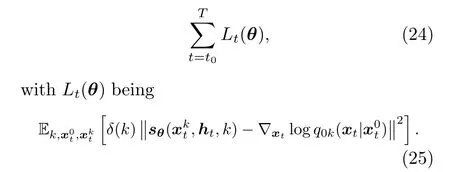
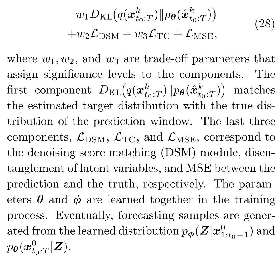
In practice, we may encounter the challenge of insufficient observations.If historical multivariate time series were recorded based on a short period,they will be prone to a significant level of noise due to measurement errors,sampling variability,and randomness from other sources.To address the problem of limited and noisy time series, D3VAE, proposed by Li Y et al.(2022), employs a coupled diffusion process for data augmentation,and then uses a bidirectional variational autoencoder (BVAE) together with denoising score matching to clear the noise.In addition, D3VAE considers disentangling latent variables by minimizing the overall correlation for better interpretability and stability of predictions.Moreover,the mean square error(MSE)between the prediction and actual observations in the prediction window is included in the objective function,further emphasizing the role of supervision.

Assuming that the prediction window can be generated from a set of latent variablesZthat follows a Gaussian distributionq(Z|x01:t0-1), the conditional distribution ofZis approximated withpφ(Z|x01:t0-1), whereφdenotes learnable parameters.Then, the forecasting time series ?xt0:Tcan be generated from the estimated target distribution,given bypθ(x0t0:T|Z).It is not difficult to see that the prediction window is still predicted based on the context window,however,with latent variablesZas an intermediate.

In the coupled diffusion process,we inject noises separately into the context window and the prediction window.Different from TimeGrad which injects noise in the observation at each time point individually, the coupled diffusion process is applied to the whole period.For the context window, the same kernel as Eq.(2)is applied such that

where∈denotes the standard Gaussian noise but with a matrix rather than a vector form.

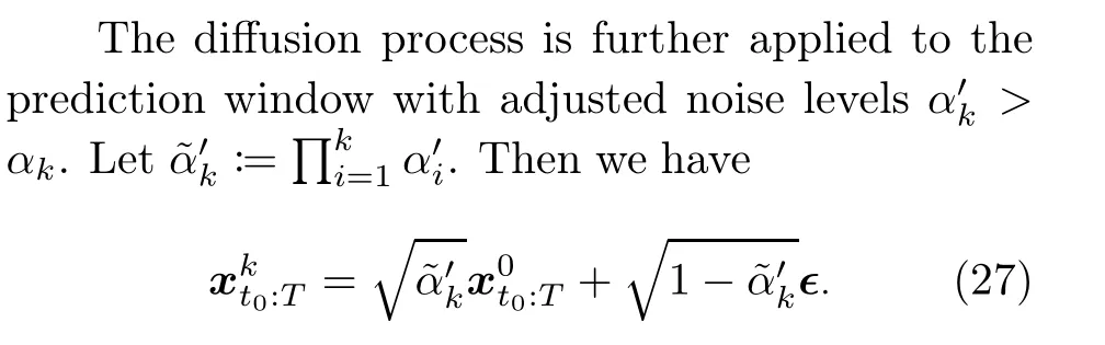
This diffusion process simultaneously augments the context window and the prediction window,thus improving the generalization ability for short-timeseries forecasting.In addition, it was proven by Li Y et al.(2022) that the uncertainty caused by the generative model and the inherent noises in the observed data can both be mitigated by the coupled diffusion process.

The backward process is accomplished with two steps.The first step is to predictxkt0:Twith a BVAE as the one used in Vahdat and Kautz (2020), which is composed of an encoder and a decoder with multiple residual blocks and takes the disturbed context windowxk1:t0-1as input.The latent variables inZare gradually generated and fed into the model in a summation manner.The output of this process is the predicted disturbed prediction window ?xkt0:T.The second step involves further cleaning of the predicted data with a denoising score-matching module.Specifically, the final prediction is obtained via a single-step gradient jump (Saremi and Hyv?rinen,2019):

whereσ0is prescribed andE(?xkt0:T;e) is the energy function.

Disentanglement of latent variablesZcan effi-ciently enhance the model interpretability and reliability for prediction (Li YN et al., 2021).It is measured by the total correlation of the random latent variablesZ.Generally, a lower total correlation implies better disentanglement and is a signal of useful information.The computation of total correlation happens synchronously with the BVAE module.

The objective function of D3VAE consists of four components.It can be written as

3.5 DSPD

Multivariate time-series data can be considered as a record of value changes for multiple features of an entity of interest.Data are collected from the same entity, and the measuring tools normally stay unchanged during the whole observed time period.So, assuming that the change of variables over time is smooth, the time-series data can be modeled as values from an underlying continuous function(Bilo? et al., 2023).In this case, the context window is expressed asX0c={x(1),x(2),...,x(t0- 1)}and the prediction window becomesX0p={x(t0),x(t0+1),...,x(T)}, wherex(·) is a continuous function of the time pointt.

Different from traditional diffusion models, the diffusion and reverse processes are no longer applied to vector observations at each time point.Alternatively, the target of interest is the continuous functionx(·), which means noises will be injected and removed from a function rather than a vector.Therefore,a continuous noise function∈(·)should take the place of the noise vector∈～N(0,I).This function should be both continuous and tractable,such that it accounts for the correlation between measurements and enables training and sampling.These requirements are effectively satisfied by designing a Gaussian stochastic process∈(·)～GP(0,Σ)(Bilo? et al.,2023).

Discrete stochastic process diffusion (DSPD) is built upon the DDPM formulation but with the stochastic process∈(·)～GP(0,Σ).It is a delight that DSPD is only slightly different from DDPM in terms of implementation.Specifically,DSPD simply replaces the commonly applied noise∈～N(0,I) with the noise function∈(·) whose discretized form is∈～N(0,Σ).LetX0be an observed multivariate time series in a certain period of timeT′={t′1,t′2,...,t′T}, which meansX0={x(t′1),x(t′2),...,x(t′T)}.In the forward process,noise is injected through the transition kernel

Then,the following backward transition kernel is applied to recover the original data:

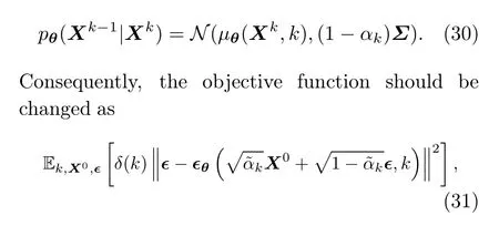
where∈～N(0,Σ)with the covariance matrix from the Gaussian processGP(0,Σ).

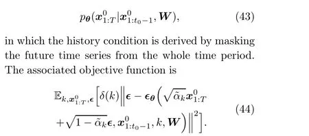
Forecasting via DSPD is very similar to TimeGrad.As before, the aim is still to learn the conditional probabilityq(X0p|X0c),but there are two major improvements.First, the prediction is available for any future time point in the continuous time interval.Second,instead of step-by-step forecasting,DSPD can generate samples for multiple time points in one run.By adding the historical condition into the fundamental objective function in Eq.(31), the objective function for DSPD forecasting is then given by

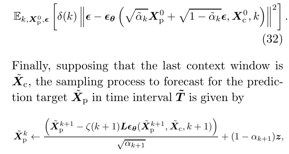
whereLis from the factorization of the covariance matrixΣ=LLT,the last diffusion output is generated as ?XKp～N(0,Σ), andz～N(0,Σ).

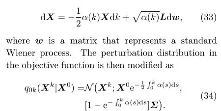
Similar to the extension from TimeGrad to ScoreGrad, the continuous noise function can be adapted to the SDE framework, thus leading to the continuous stochastic process diffusion (CSPD)model (Bilo? et al., 2023).The diffusion process of CSPD introduces the factorized covariance matrixΣ=LLTto the VP SDE (see Section 2.4)as

3.6 TimeDiff

TimeGrad adopts the autoregressive sampling process, in which the prediction of the former time point should be sent back to the encoding algorithm to compute the condition for sampling the next prediction.Therefore, errors can accumulate with the increase of prediction interval length, restricting TimeGrad’s ability to forecast long-term time series.In addition, the autoregressive sampling process is very slow compared to one-shot generative methods (i.e., methods that generate the prediction for the whole prediction interval in one run).To solve these problems, a non-autoregressive method called TimeDiffwas proposed(Shen and Kwok,2023).

In TimeGrad, the condition of target conditional distribution is the hidden states of the history window obtained via an RNN module.Alternatively, TimeDiffcombines two sources of information as the condition, including a future mixup and a future approximation.Future mixup, inspired by Zhang HY et al.(2018), integrates past and future information at each diffusion stepkvia a random maskmk ∈[0,1)D×(T-t0+1)sampled from the uniform distribution on[0,1)as follows:

where Conv(·)is a convolution network for encoding local temporal patterns and long-term dependencies.In the sampling process,where the future values are unknown,the mixup is simply set as

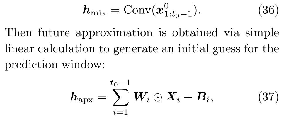
whereXi ∈RD×(T-t0+1)is a matrix of(T-t0+1)copies ofx0i, andWiandBiare learnable matrices.The future approximation is actually a linear autoregressive model, which can reduce the disharmony between the history and prediction windows (Lugmayr et al., 2022; Shen and Kwok, 2023).However,this model does not require autoregressive sampling because it is based only on historical information.Hence, TimeDiffeffectively avoids the error accumulation and slow sampling caused by the autoregressive mechanism.The last step to construct the condition is to vertically concatenate future mixup and future approximation as Instead of approximating the noise injected at each diffusion step, TimeDiff’s objective function aims to approximate the original data directly.It is assumed that the mean of the reverse transition kernel in Eq.(3)is alternatively approximated withxθrather than∈θas

Accordingly, this mean is also applied in the sampling process with the learned data matching networkxθ.

3.7 DiffSTG

Spatio-temporal graphs (STGs) are a special type of multivariate time series that encodes spatial and temporal relationships and interactions among different entities in a graph structure (Wen et al.,2023).They are commonly observed in real-life applications such as traffic flow prediction(Li YG et al.,2018) and weather forecasting (Simeunovi? et al.,2022).Suppose we haveNentities of interest,such as traffic sensors or companies in the stock market.We can model these entities and their underlying relationships as a graphG={V,E,W},whereVis a set ofNnodes as representations of entities,Eis a set of links that indicates the relationship between nodes,andWis a weighted adjacency matrix that describes the graph topological structure.Multivariate time series observed at all entities are models as graph signalsX0c={x01,x02,...,x0t0-1|x0t ∈RD×N}, which means we haveD-dimensional observations fromNentities at each time pointt.A visualized illustration of STGs is provided in Fig.3.Identical to the previous problem formulation,the aim of STG forecasting is to predictX0p={x0t0,x0t0+1,...,x0T|x0t ∈RD×N}based on the historical informationXc.Nevertheless, except for the time dependency on historical observations,we also need to consider the spatial interactions between different entities represented by the graph topology.

DiffSTG applies diffusion models on STG forecasting with a graph-based noise-matching network called UGnet(Wen et al.,2023).The idea of DiffSTG can be regarded as the extension of DDPM-based forecasting to STGs with an additional condition on the graph structure, which means the target distribution in Eq.(17)is approximated alternatively by

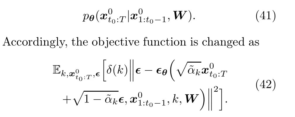
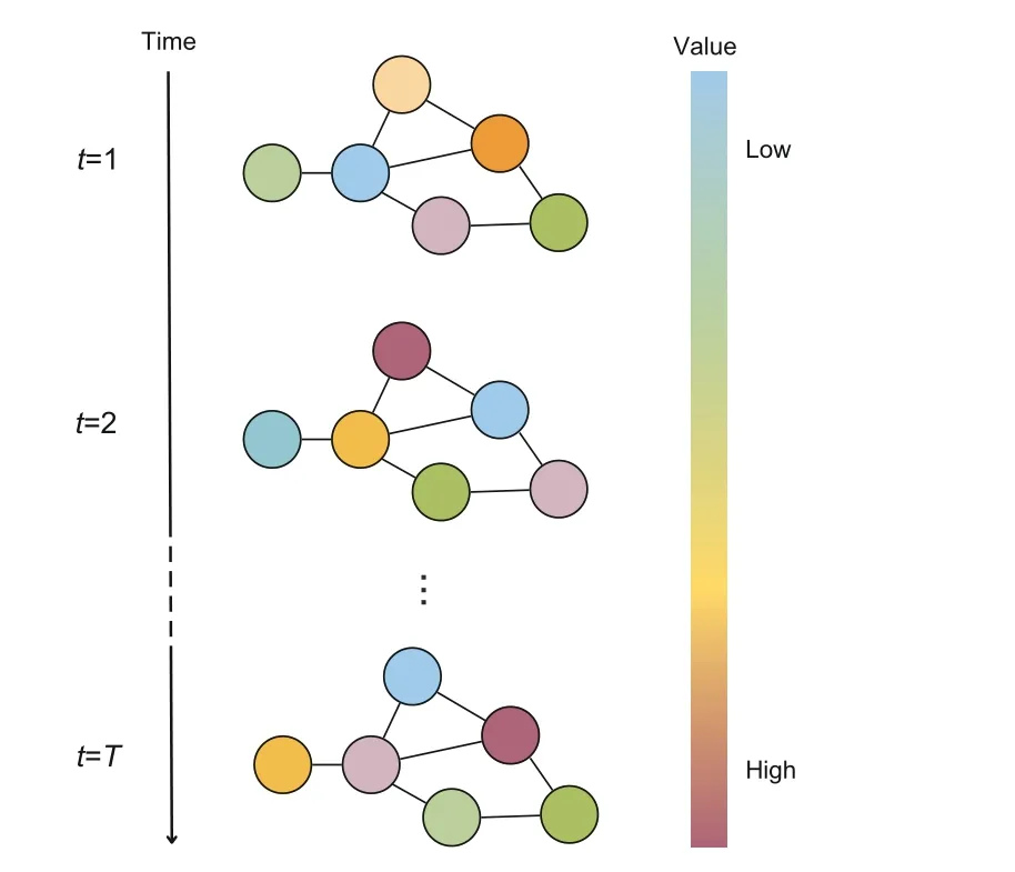
Fig.3 Illustration of spatio-temporal graphs

The objective function in Eq.(42) actually treats the context window and the prediction window as samples from two separate sample spaces,namely,X0c∈XcandX0p∈XpwithXcandXpbeing two individual sample spaces.However, considering the fact that the context and prediction intervals are consecutive,it may be more reasonable to treat the two windows as a complete sample from the same sample space.To this end, Wen et al.(2023)reformulated the forecasting problem and revised the approximation in Eq.(41)as

The training process is quite straightforward and follows common practice, but note that the sample generated in the forecasting process includes both historical and future values.So,we need to take out the forecasting target in the sample as the prediction.

Now,there is only one remaining problem.How to encode the graph structural information in the noise-matching network∈θ? Wen et al.(2023) proposed UGnet, a U-Net-based network architecture(Ronneberger et al., 2015) combined with a graph neural network (GNN) to process time dependency and spatial relationships simultaneously.UGnet takesxk1:T,x01:t0-1,kandWas inputs and then outputs the prediction of the associated error∈.

3.8 GCRDD

The graph convolutional recurrent denoising diffusion (GCRDD) model is another diffusion-based model for STG forecasting (Li RK et al., 2023).It differs from DiffSTG in that it uses hidden states from a recurrent component to store historical information as TimeGrad and employs a different network structure for the noise-matching term∈θ.Note that the notations related to STGs here follow Section 3.7.

GCRDD approximates the target distribution with a probabilistic density function conditional on the hidden states and graph structure as follows:

where the hidden state is computed with a graphmodified GRU, written as

The graph-modified GRU replaces the weight matrix multiplication in a traditional GRU (Chung et al.,2014)with graph convolution such that both temporal and spatial information is stored in the hidden state.The objective function of GCRDD adopts a similar form of TimeGrad but with additional graph structural information in the noise-matching network:

For the noise-matching term,GCRDD adopts a variant of DiffWave(Kong et al.,2021)that incorporates a graph convolution component to process spatial information inW.STG forecasting via GCRDD is the same as TimeGrad except that the sample generated at each time point is a matrix rather than a vector.

4 Time-series imputation

In real-world problem settings, we usually encounter the challenge of missing values.When collecting time-series data, the collection conditions may change over time, which makes it difficult to ensure the completeness of observation.In addition, accidents such as sensor failures and human errors may result in missing historical records.Missing values in time-series data normally have a negative impact on the accuracy of analysis and forecasting because the lack of partial observations makes the inference and conclusions vulnerable in future generalization.

Time-series imputation aims to fill in the missing values in incomplete time-series data.Many previous studies have focused on designing deep learning based algorithms for time-series imputation(Osman et al., 2018).Most existing approaches involve the RNN architecture to encode time dependency in the imputation task (Cao et al., 2018; Che et al., 2018;Luo YH et al., 2018; Yoon et al., 2019).Except for these deterministic methods, probabilistic imputation models such as GP-VAE (Fortuin et al., 2020)and V-RIN (Mulyadi et al., 2022) have shown their practical value in recent years.As a rising star in probabilistic models,diffusion models have also been applied to time-series imputation tasks (Tashiro et al., 2021; Alcaraz and Strodthoff, 2023).Compared with other probabilistic approaches,diffusionbased imputation enjoys high flexibility in the assumption of the true data distribution.In this section, we will cover four diffusion-based methods, including three for multivariate time-series imputation and one for STG imputation.

4.1 Problem formulation

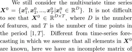
Note that the problem formulation here is only a typical case.Later, in Section 4.4, we will introduce another formulation that takes the whole time-series matrixX0as the target for generation.

4.2 CSDI

Conditional-score-based diffusion model for imputation(CSDI)is the pioneering work on diffusionbased time-series imputation (Tashiro et al., 2021).Identical to TimeGrad, the basic diffusion formulation of CSDI is DDPM.However,as we discussed in Section 3.2, the historical information is encoded by an RNN module in TimeGrad, which hampers the direct extension of TimeGrad to imputation tasks because the computation of hidden states may be interrupted by missing values in the context window.

CSDI applies the diffusion and reverse processes to the matrix of missing data,X0ms.Correspondingly, the reverse transition kernel is refined as a probabilistic distribution conditional onX0ob:

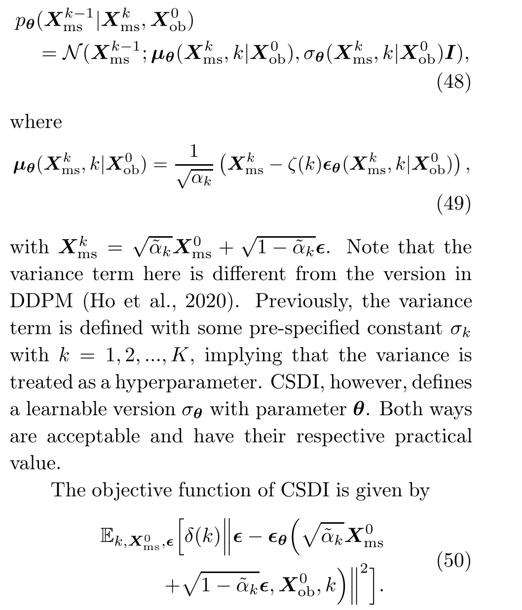
whereZ～N(0,I) fork=K-1,K-2,...,1, andZ=0 fork=0.

4.3 DSPD

Here we discuss the simple extension of DSPD and CSPD in Section 3.5 to time-series imputation tasks.Because the rationale behind the extension of these two models is almost identical, we focus only on DSPD for illustration.The assumption of DSPD states that the observed time series is formed by values of a continuous functionx(·)of timet.Therefore,the missing values can be obtained by computing the values of this continuous function at the corresponding time points.Recall that DSPD uses the covariance matrixΣinstead of the DDPM varianceσkIorσθin the backward process.Therefore,one may apply DSPD to imputation tasks in a manner similar to CSDI by replacing the variance term in Eq.(48)with the covariance matrixΣ.According to Bilo? et al.(2023), the continuous noise process is a more natural choice than the discrete noise vector because it takes account of the irregularity in the measurement when collecting the time-series data.

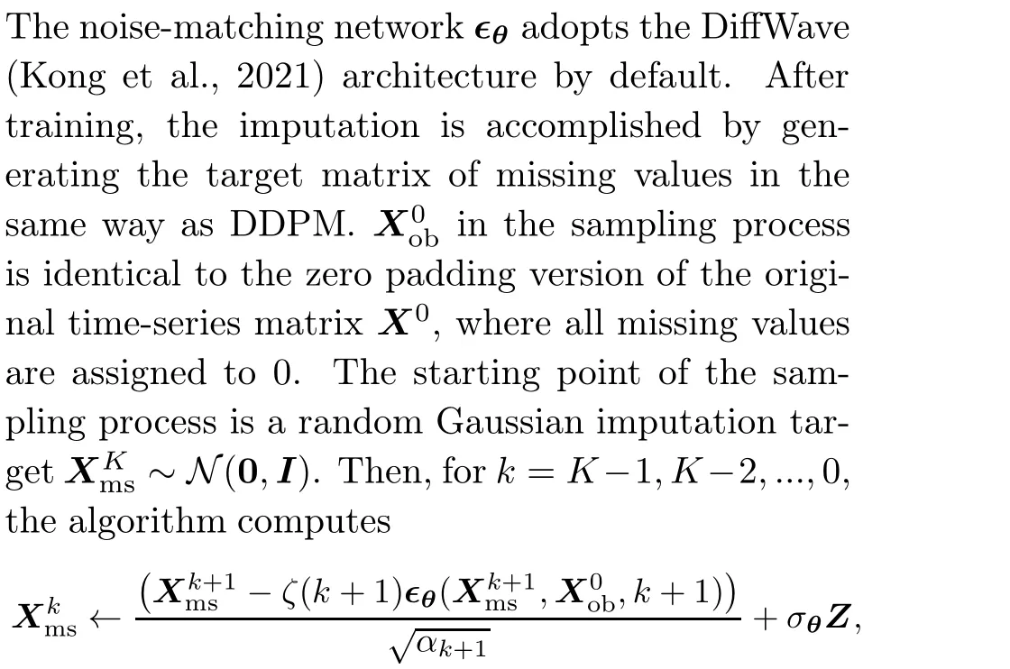
4.4 SSSD

Structured state space diffusion (SSSD) differs from the aforementioned two methods by having the whole time-series matrixX0as the generative target in its diffusion module (Alcaraz and Strodthoff,2023).The name,“structured state space diffusion,”comes from the design of the noise-matching network∈θ, which adopts the state space model (Gu et al.,2022) as the internal architecture.As a matter of fact,∈θcan also take other architectures such as the DiffWave-based network in CSDI(Tashiro et al.,2021) and SaShiMi, a generative model for sequential data (Goel et al., 2022).However, the authors of SSSD have shown empirically that the structured state space model generally generates the best imputation outcome compared with other architectures(Alcaraz and Strodthoff, 2023).To emphasize the difference between this method and other diffusionbased approaches, we primarily focus on the unique problem formulation used by SSSD.

As we mentioned,the generative target of SSSD is the whole time-series matrix,X0∈RD×T, rather than a matrix that particularly represents the missing values.For the purpose of training,X0is also processed with zero padding.The conditional information, in this case, is from a concatenated matrixX0c= Concat(X0⊙Mc,Mc), whereMcis a 0-1 matrix indicating the position of observed values as the condition.The element inMccan only be 1 if its corresponding value inX0is known.

There are two options for the objective function used in the training process.Similar to other approaches, the objective function can be a simple conditional variant of the DDPM objective function:

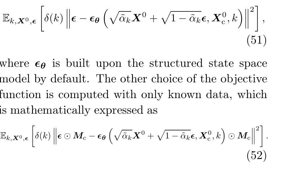
According to Alcaraz and Strodthoff(2023),the second objective function is typically a better choice in practice.For forecasting, SSSD employs the usual sampling algorithm and applies to the unknown entries inX0, namely, (1-Mc)⊙X0.

An interesting point proposed along with SSSD is that imputation models can also be applied to forecasting tasks.This is because future time series can be viewed as a long block of missing values on the right ofX0.Nevertheless, experiments have shown that the diffusion-based approaches underperform other methods such as the autoformer(Wu et al., 2021)in forecasting tasks.

4.5 PriSTI

PriSTI is a diffusion-based model for STG imputation (Liu MZ et al., 2023).However, different from DiffSTG, the existing framework of PriSTI is designed for STGs with only one feature,which means the graph signal has the formX0={x01,x02,...,x0T}∈RN×T.Each vectorx0t ∈RNrepresents the observed values ofNnodes at time pointt.This kind of data is often observed in traffic prediction(Li YG et al., 2018)and weather forecasting(Yi et al.,2016).METR-LA,for example,is an STG dataset that contains traffic speed collected by 207 sensors on a Los Angeles highway in a four-month time period (Li YG et al., 2018).There is only one node attribute, that is, traffic speed.However, unlike the multivariate time-series matrix, where features (sensors in this case) are usually assumed to be uncorrelated,the geographic relationship between different sensors is stored in the weighted adjacency matrixW,allowing a more pertinent representation of real-world traffic data.

The number of nodesNcan be considered as the number of featuresDin CSDI.The only difference is that PriSTI incorporates the underlying relationship between each pair of nodes in the conditional information for imputation.So, the problem formulation adopted by PriSTI is the same as our discussion in Section 4.1, and thus the goal is still to findq(X0ms|X0ob).

To encode graph structural information, the mean in Eq.(49)is modified as

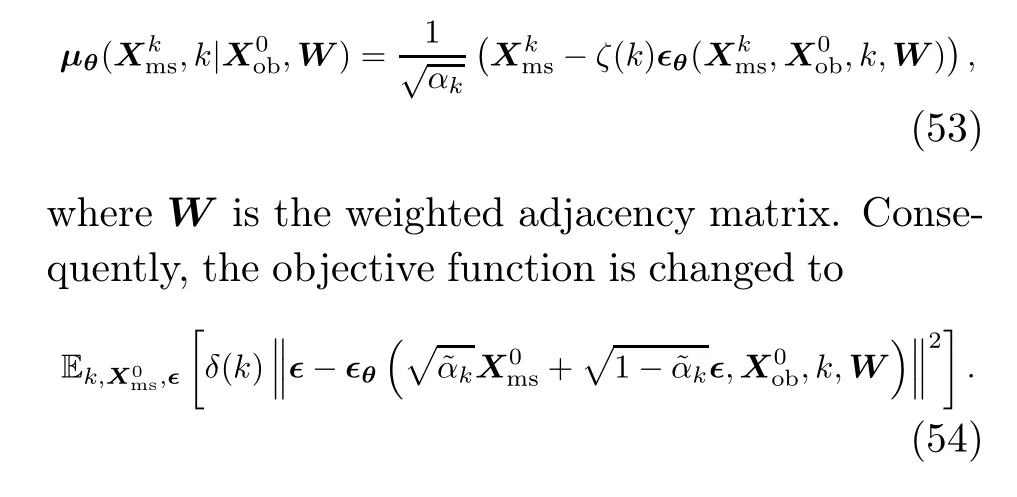
The conditional information,X0ob, is processed with linear interpolation before it is fed into the algorithm to incorporate extra noises, which will enhance the denoising capability of the model and eventually lead to better consistency in prediction(Choi et al.,2022).The noise-matching network∈θis composed of two modules, including a conditional feature extraction module and a noise estimation module.The conditional feature extraction module takes the interpolated informationX0oband adjacency matrixWas inputs and generates a global context with both spatial and temporal information as the condition for diffusion.Then, the noise estimation module uses this global context to estimate the injected noises with a specialized attention mechanism to capture temporal dependencies and geographic information.Ultimately, the STG imputation is fulfilled with the usual sampling process of DDPM, but with the specially designed noise-matching network here to incorporate the additional spatial relationship.

Because PriSTI works only for the imputation of STGs with a single feature, which is simply a special case of STGs, this model’s practical value is somewhat limited.So, the extension of the idea here to more generalized STGs is a notable topic for future researchers.

5 Time-series generation

The rapid development of the machine learning paradigm requires high-quality data for different learning tasks in finance, economics, physics, and other fields.The performance of the machine learning model and algorithm may be highly subject to the underlying data quality.Time-series generation refers to the process of creating synthetic data that resembles the real-world time series.Because the time-series data are characterized by their temporal dependencies, the generation process usually requires the learning of underlying patterns and trends from past information.

Time-series generation is a developing topic in the literature and several methods exist(Yoon et al.,2019; Desai et al., 2021).Time-series data can be seen as a case of sequential data, whose generation usually involves the generative adversarial network(GAN) architecture (Mogren, 2016; Esteban et al.,2017;Donahue et al.,2019;Xu TL et al.,2020).Accordingly, TimeGAN is proposed to generate timeseries data based on an integration of RNN and GAN for the purpose of processing time dependency and generation (Yoon et al., 2019).However, the GANbased generative methods have been criticized because they are unstable (Chu et al., 2020) and subject to the model collapse issue (Xiao et al., 2022).Another way to generate time-series data stems from the VAE, leading to the so-called TimeVAE model (Desai et al., 2021).As a common shortcoming of VAE-based models, TimeVAE requires a user-defined distribution for its probabilistic process.Here we present a different probabilistic time-series generator that originates from diffusion models and is more flexible with the form of the target distribution (Coletta et al., 2023; Lim et al., 2023).This section aims to enlighten researchers about this new research direction,and we expect to see more derivative works in the future.

5.1 Problem formulation

With the multivariate time seriesX0={x01,x02,...,x0T|x0i ∈RD}, the time-series generation problem aims to synthesize time seriesx01:Tin the same time period.The problem formulation may vary in different papers.Here, we will focus on two different methods,conditional score based timeseries generative model (TSGM) (Lim et al., 2023)and TimeDiff(Coletta et al., 2023).TSGM synthesizes time series by generating observationx0tat time pointt ∈[2,T]with the consideration of its previous historical datax01:t-1.Correspondingly, the target distribution is the conditional densityq(x0t|x01:t-1)fort ∈[2,T], and the associated generative process involves the recursive sampling ofxtfor all time points in the observed period.With DiffTime,alternatively, time-series generation is formed as a constrained optimization problem, and the condition in target distribution is designed based on specific constraints rather than just historical information.Details about the training and generation processes will be discussed in the following subsections.

5.2 TSGM

TSGM was proposed to conditionally generate each time-series observation based on the past generated observations(Lim et al.,2023).The TSGM architecture includes three components: an encoder,a decoder, and a conditional score-matching network.The pre-trained encoder is used to embed the underlying time series into a latent space.The conditional score-matching network is used to sample the hidden states, which are then converted to the time-series samples via the decoder.

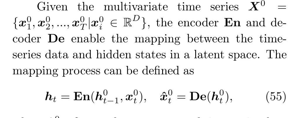
Given the auto-dependency characteristic of the time-series data, learning the conditional loglikelihood function is essential.To address this,the conditional score-matching network is designed based on the SDE formulation of diffusion models.Note that TSGM focuses on the generation of hidden states rather than producing the time series directly with the sampling process.At time stept, instead of applying the diffusion process tox0t, the hidden stateh0tis diffused to a Gaussian distribution by the following forward SDE:

wherek ∈[0,K]refers to the integral time.With the diffused sampleh, the conditional score-matching networksθlearns the gradient of the conditional log-likelihood function with the following objective function:

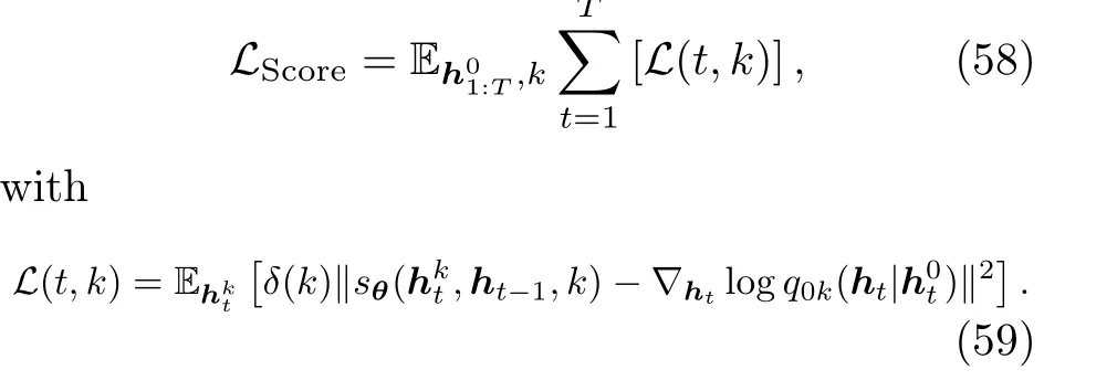
The network architecture ofsθis designed based on U-Net(Ronneberger et al.,2015),which was adopted by the classic SDE model (Yang S et al.,2021).

In the training process,the encoder and decoder are pre-trained using the objectiveLED.They can also be trained simultaneously with the networksθ,but Lim et al.(2023) showed that the pre-training generally led to better performance.Then, to learn the score-matching network, hidden states are first obtained through inputting the entire time seriesx01:Tinto the encoder,and then fed into the training algorithm with the objective functionLScore.The time-series generation is achieved by sampling hidden states and then applying the decoder,where the sampling process is analogous to solving the timereverse SDE.

The TSGM method can achieve state-of-theart sampling quality and diversity, compared to a range of well-developed time-series generation methods.However, it is still subject to the fundamental limitation that all diffusion models may have-they are generally more computationally expensive than GANs.

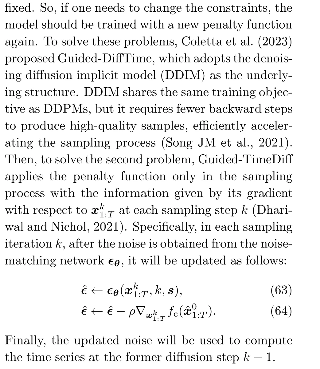
5.3 DiffTime, Loss-DiffTime, and Guided-DiffTime

Sometimes synthetic time series are required to be statistically similar to historical time series but involve some specific constraints.For example, synthetic energy data are expected to follow the principle of energy conservation(Seo et al., 2021).Hence,Coletta et al.(2023) proposed DiffTime to handle the constrained time-series generation problem.

TimeDiffconsiders two types of constraints,the trend constraint as a time seriess ∈RD×Tand the fixed-point constraint on a specific variable at a certain time point.To incorporate the trend constraint,

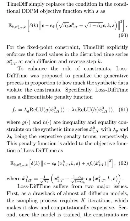
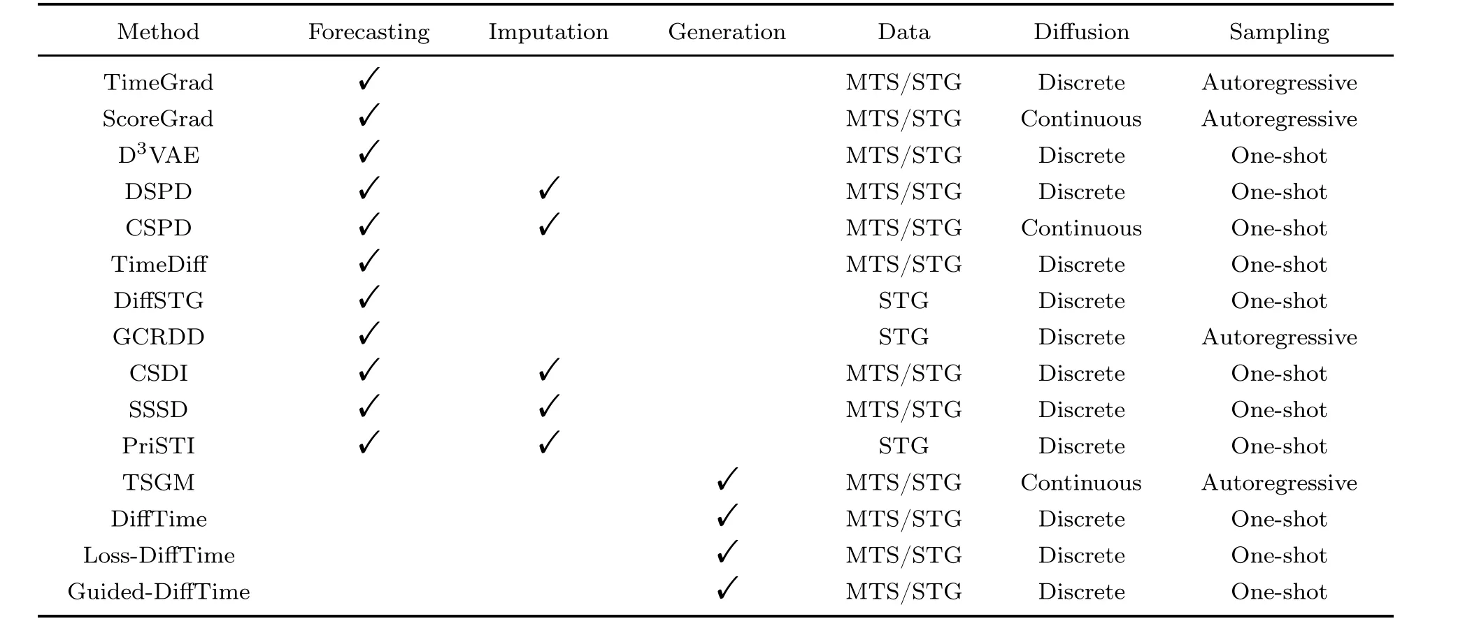
Table 2 Comparison of diffusion models for time-series applications

6 Model comparison

In Table 2, we provide a comparison of all 15 methods mentioned in this review.We compare the time-series tasks that each model can conduct.Although most models were designed specifically for one of the three tasks, some of them can be applied to multiple tasks by nature.Specifically, models for imputation can be applied to forecasting tasks by regarding the future time series as missing values.In addition,we compare the data types that each model can handle.Generally, models designed for multivariate time series can be extended to STG tasks by simply discarding the graph structure.However,practically,the performance of these models on STG datasets may not be satisfactory.We also compare the diffusion process of different models,categorizing them into discrete diffusion and continuous diffusion.Most models with discrete diffusion are based on the DDPM formulation (Ho et al., 2020), while models with continuous diffusion follow the SDE-based design (Yang S et al., 2021).Finally, we consider the distinctions in the sampling process.Specifically,we categorize the models as either autoregressive generators or one-shot generators.With the autoregressive sampling process, models produce predictions for one time point in one sampling iteration.By contrast,one-shot models generate full time series for the whole target time period in one run.Normally,autoregressive methods are more accurate, but oneshot generation is more computationally efficient because it requires only one sampling iteration (Wen et al., 2023).

7 Practical applications

To highlight the practical value of diffusion models for time series, we provide a brief review of relevant real-world applications.In general, diffusion models can be applied to almost all kinds of timeseries-based problems, because most are designed to handle broad time-series forecasting, imputation,and generation tasks.In this section, we delve into some primary application domains, and our discussion is divided into two subsections depending on the data type.Specifically,we focus on general timeseries and STG applications.Although there can be an overlap between the applications of these two data types because STGs are special cases of multivariate time series, studies in these two areas usually have different emphases.

7.1 General time-series applications

The study of diffusion models for time series involves data from numerous real-world application domains.Because diffusion models are highly flexible and can generate data from any distribution,they can be used to generate time-series data with complicated patterns and dependencies.Specifically, when the data are subject to high uncertainty by nature,diffusion models can generate probabilistic outputs to better represent the uncertainty, leading to better insights and decisions(Capel and Dumas, 2023).Here we will present two frequently discussed examples from the literature,including energy forecasting and medical practices.

7.1.1 Energy forecasting

Energy forecasting is of essential importance for decision-making in environment control, energy management, and power distribution.For example,renewable energy forecasting helps enhance the operational predictability of modern power systems,contributing to the control of energy mix for consumption, and eventually, leading to better control of carbon emissions and climate change.However,renewable energies such as solar energy and wind energy are affected by external factors such as unexpected natural conditions, resulting in unstable production and consumption.To capture the uncertainty in renewable energy generation,Capel and Dumas (2023) proposed to use DDPMs for renewable energy forecasting and showed the superiority of DDPMs in terms of accuracy over other generative methods.As another example, Wang et al.(2023)proposed DiffLoad,a diffusion-based Seq2Seq structure,for electricity load forecasting that will ultimately contribute to the planning and operation of power systems.

7.1.2 Medical practices

To meet increasing requirements, analysis of physiological signals has become crucial (Zhang YF et al.,2021).In clinical settings,an accurate predictive model is important for detecting potential unusual signals.The transform-based diffusion probabilistic model for sparse time-series forecasting(TDSTF),a transformer-based diffusion model,was proposed for heart rate and blood pressure forecasting in the intensive care unit (ICU) and shown as an effective and efficient solution compared to other models in the field (Chang et al., 2023).In addition, diffusion models can be designed for electroencephalogram (EEG) and electrocardiogram (ECG)signal prediction, imputation, and generation,offering valuable support for clinical treatments(Neifar et al.,2023;Shu et al.,2023).

7.2 Spatial temporal graph applications

STGs are a special type of multivariate timeseries data that record the change of values of one or multiple variables of different entities in a system over time.The literature on diffusion models for STGs covers two application domains, transportation (Li RK et al., 2023; Wen et al., 2023) and air quality monitoring (Liu MZ et al., 2023;Wen et al.,2023).

7.2.1 Transportation

For transportation, the system of interest is usually traffic networks with numerous sensors that monitor traffic conditions and collect traffic data such as vehicle speed and traffic flow(Xu DW et al.,2017;Seng et al.,2021).In traffic STGs,graph nodes are traffic sensors,and edges are usually constructed based on the geometric distance between each pair of sensors.Given the record of historical traffic data,the objective of traffic forecasting is to predict the average traffic speed or traffic flow in the next time period (e.g., an hour) for all sensors.Existing diffusion models serving this purpose include DiffSTG(Wen et al.,2023)and GCRDD(Li RK et al.,2023).Diffusion models can also be used for traffic data imputation(Liu MZ et al.,2023).Due to sensor failures or human errors, missing records are common in traffic data, which causes issues in analysis and prediction (Yi et al., 2016); thus, diffusion models can be applied to predict the missing values before forwarding the data for further analysis.

7.2.2 Air quality monitoring

Diffusion models have also been applied to address air quality problems,including air quality prediction and air data imputation.In such tasks, air monitoring stations are modeled as graph nodes,and the edges are also formed based on geometric information.The objectives of air quality prediction and air data imputation are analogous to traffic forecasting and imputation.For example,PM2.5prediction,one of the famous tasks in this application domain,aims to predict future PM2.5readings of several air monitoring stations in a city (Yi et al., 2018; Wen et al., 2023).

7.3 Publicly available datasets

In Table 3,we list some frequently used publicly available datasets in the study of diffusion models for time series.We present datasets from papers focusing on either multivariate time series or STGs.We also categorize the datasets by their application domains and provide their source links.With high data quality, public availability, and close reflection of real-world implications,these datasets can serve as valuable resources for researchers and practitioners to test and understand diffusion models in various application domains.

8 Future research directions

Up to this point, we have discussed different methods for time-series forecasting,imputation,generation, and some relevant practical application domains.Now, we look into the limitations of existing models and challenges in this research area that may lead to future research directions and inspire future researchers.

1.Heavy model selection

How to select the optimal diffusion model structure still remains an open problem.Designing a diffusion model for time series requires the selection of many building blocks, such as the condition, the noise-matching network or other networks serving similar purposes,and the sampling acceleration technique.However,there are many potential choices for these building blocks without a unified framework or criterion for evaluation.For example, to construct a good condition for the target distribution, how to represent a time series effectively is quite essential(Yin et al., 2015).While TimeGrad (Kashif et al.,2021)and GCRDD(Li RK et al.,2023)choose RNN to encode historical information as the condition,other serial data encoders such as the transformer encoder (Vaswani et al., 2017) can be adopted to boost good performance as well(Sikder et al.,2023).For each building block, the choice is highly flexible but suffers from heavy tuning costs of structures and hyperparameters.This highlights the importance of research on the comparison of different options and a unified framework or guidance on model selection.

2.Insufficient research on noise injection

Noise injection, as an important component of diffusion models,has not been sufficiently studied in the research for time series.First, current researchconsiders only injecting Gaussian noise,leaving lack of study on other distributions and noises designed specifically for discrete time-series data.In addition,the noise schedule (i.e., howαkchanges with the diffusion steps) is not carefully designed for timeseries data.Currently, we can observe research only on the noise schedule for images(Chen, 2023).

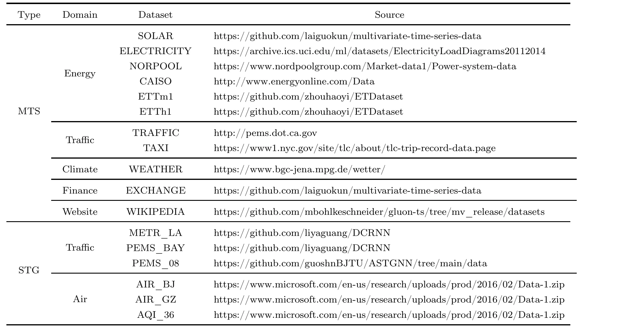
Table 3 Publicly available datasets of multivariate time series (MTS) and spatio-temporal graphs (STG)

3.Unsatisfactory performance with spatiotemporal graphs

Although there are several studies on diffusion models for STG forecasting,the performance of these models is still unsatisfactory.Specifically, diffusion models fail to outperform the deterministic methods such as DCRNN (Li YG et al., 2018) and GMSDR(Liu DC et al., 2022).To enhance performance, one may consider how to better encode the spatial information in diffusion models.Currently, the graph structureWis used only as part of the condition,so how to enhance the role of spatial information is still a problem to be solved.Moreover,exiting diffusion models for STGs are very slow at sampling (Li RK et al., 2023).This shows the need for designing or incorporating suitable sampling acceleration techniques.

9 Conclusions

Diffusion models, a rising star in advanced generative techniques, have shown their exceptional power in various real-world applications.In recent years, many successful attempts have been made to incorporate diffusion in time-series applications to boost model performance.As compensation for the lack of a methodical summary and discourse on diffusion-based approaches for time series, we have furnished a self-contained survey of these approaches while discussing the interactions and differences among them.Specifically, we have presented seven models for time-series forecasting, four models for time-series imputation, and four models for time-series generation.Although these models have shown good performance with empirical evidence,we feel obligated to emphasize that they are usually associated with very high computational costs.In addition, because most models are constructed with a high level of theoretical background,there is still a lack of deeper discussion and exploration of the rationale behind these models.This survey is expected to serve as a starting point for new researchers in this area and inspiration for future directions.

Contributors

Junbin GAO initialized the idea.Lequan LIN collected all relevant literature for review and created all the figures and tables.Lequan LIN and Zhengkun LI drafted the paper.Ruikun LI and Xuliang LI helped organize the paper.All authors revised and finalized the paper.

Compliance with ethics guidelines

Junbin GAO is a guest editor of this special feature,and he was not involved with the peer review process of this paper.Lequan LIN, Zhengkun LI, Ruikun LI, Xuliang LI, and Junbin GAO declare that they have no conflict of interest.