Surface Weather Parameters Forecasting Using Analog Ensemble Method over the Main Airports of Morocco

ABSTRACT Surface weather parameters detain high socioeconomic impact and strategic insights for all users, in all domains(aviation, marine traffic, agriculture, etc.). However, those parameters were mainly predicted by using deterministic numerical weather prediction (NWP) models that include a wealth of uncertainties. The purpose of this study is to contribute in improving low-cost computationally ensemble forecasting of those parameters using analog ensemble method (AnEn) and comparing it to the operational mesoscale deterministic model (AROME) all over the main airports of Morocco using 5-yr period (2016–2020) of hourly datasets. An analog for a given station and forecast lead time is a past prediction, from the same model that has similar values for selected predictors of the current model forecast. Best analogs verifying observations form AnEn ensemble members. To picture seasonal dependency, two configurations were set; a basic configuration where analogs may come from any past date and a restricted configuration where analogs should belong to a day window around the target forecast. Furthermore, a new predictors weighting strategy is developed by using machine learning techniques (linear regression, random forest, and XGBoost). This approach is expected to accomplish both the selection of relevant predictors as well as finding their optimal weights,and hence preserve physical meaning and correlations of the used weather variables. Results analysis shows that the developed AnEn system exhibits a good statistical consistency and it significantly improves the deterministic forecast performance temporally and spatially by up to 50% for Bias (mean error) and 30% for RMSE (root-mean-square error) at most of the airports. This improvement varies as a function of lead times and seasons compared to the AROME model and to the basic AnEn configuration. The results show also that AnEn performance is geographically dependent where a slight worsening is found for some airports.

Key words: analog ensemble, machine learning, surface weather parameters, ensemble forecasting, AROME (Applications de la Recherche à l’Opérationnel à Méso-Echelle), predictors weighting strategy

1. Introduction

In most national meteorological services, numerical weather prediction (NWP) is mainly based on determinism. In this doctrine, given an initial state of the atmosphere, its evolution numerically leads to a unique prediction scenario. However, deterministic weather forecasts show several uncertainties, occasioned by several error sources related to model formulation (Orrell et al.,2001), initial state (PaiMazumder and M?lders, 2009),physical parameterization (Palmer, 2001), and lateral boundary conditions (Eckel and Mass, 2005). In front of those limitations, ensemble prediction takes advantage of all these uncertainty sources to construct multiple forecasts starting from slightly different but equally-probable initial states (Leith, 1974). Several national weather services around the world use ensemble prediction systems such as the NCEP (Toth and Kalnay, 1993, 1997;Toth, 2001; Zhu, 2005; Zhou et al., 2017), ECMWF(Buizza, 2008; Buizza and Richardson, 2017), the Meteorological Service of Canada (Buizza et al., 2005), and Météo-France (Vié et al., 2011). Those systems exhibit a high efficiency helping forecasters of those centers in the decision-making process. In order to construct ensemble prediction systems, several techniques were deployed such as perturbative methods that depend on atmospheric flow and based on perturbations in sub-spaces where initial condition errors grow faster, for example: breeding vectors (Toth and Kalnay, 1993, 1997) and singular vectors (Molteni et al., 1996). Recently, new data assimilation methods emerged and are included in ensemble systems for NCEP (Whitaker et al., 2008; Zhou et al., 2017)and for ECMWF (Hamill et al., 2000, 2011; Buizza et al.,2008).

Among those techniques, analog ensemble (hereafter AnEn) forecasting is considered as an intuitive and low cost method of generating ensemble members. The fundamental idea of this method is to construct an ensemble forecast from a set of past observations of the variable to be predicted, neatly selected from a historical training dataset. For a given location, the most similar past forecasts to the current prediction are identified and their associated past observations are nominated as members of the analog forecast ensemble. Thus, the availability of records of NWP deterministic forecasts is a cornerstone to the application of this method. Analog ensemble method’s objective is to discern all the past weather conditions where the error probability density function was similar.Once those conditions are distinguished, one can use the past observation errors to deduce the future errors probability density function. Analog ensemble method was theoretically introduced firstly by Hamill and Whitaker(2006), and then, it was successfully applied by Delle Monache et al. (2013), hereafter DM13, to generate probabilistic prediction of wind at 10 m and temperature at 2 m. Then, several successful applications of this technique chained mainly in renewable energy for wind and solar energy (Alessandrini et al., 2015; Davò et al.,2016), energy load (Alessandrini et al., 2015), tropical cyclones intensity (Alessandrini et al., 2018), air quality predictions (Djalalova et al., 2015; Delle Monache et al.,2018), dynamical forecast errors correction (Yu et al.,2014; Gong et al., 2016), and also in the field of data assimilation (Lguensat et al., 2017). However, the previous studies focused on a few surface weather parameters.These parameters represent an important aspect of meteorology because they are the basis for all weather safety messages, weather forecasts, and weather warnings worldwide. Thus, extending research studies to assess the potential of AnEn method for more surface weather forecasting (e.g., 2-m relative humidity and mean sea level pressure, zonal and meridional 10-m wind components)is still needed.

It is evident that the likelihood of finding good analogs depends strongly on the similarity metric and also the neighboring criteria (time window) and the weighting strategy applied to the predictors that exhibit correlations to the predictand. Several weighting algorithms of different philosophies were explored. The ultimate goal of these algorithms is to attribute a weight to each predictor in the AnEn method (Delle Monache et al., 2013).Junk et al. (2015) developed a static and dynamic weighting strategy where predictors weights are defined by probabilistic score minimization process over all plausible weights combinations, given discrete weight values. These strategies revealed an improvement of up to 20% in the performance of AnEn compared to the basic algorithm of DM13 where weights were initiated to 1(all predictors have the same weight). On the other hand,Gensler et al. (2016) introduced a weight optimization wrapper technique based on the Nelder–Mead simplex algorithm (Lagarias et al., 1998). The main idea of this approach is to find the best weights combination selected randomly, which minimizes the root-mean-square error (RMSE) between AnEn forecasts and actual measurements. This method outperforms the DM13 strategy by 10% to 21%. Finally, Tuba and Bottyán (2018) explored another family of weighting methods, based on AHP(Analytic Hierarchy Process) decision-making algorithm(Saaty, 1987). This method reproduces the best weights combination based on eigenvector decomposition of a matrix of ratios. Those ratios translate the importance of each variable relatively to others. Weights in this method are represented by the normalized eigenvector associated with the maximal eigenvalue. A novelty in our study is the usage of machine learning techniques to compute the predictors weights. This strategy is investigated and evaluated against traditional statistical method (linear regression). In addition, in this study we extend the target predictands and predictors to eight surface weather parameters: temperature and relative humidity at 2 m, surface and mean sea level pressure, wind speed and direction at 10 m, and also the zonal and meridional 10-m wind components.

It is to mention that this work is the first AnEn application using mesoscale operational model AROME (Applications de la Recherche à l’Opérationnel à Méso-Echelle) (Seity et al., 2011). The latter is widely used among an important part of the scientific community, and it is also used operationally in many countries, including Morocco (Hdidou et al., 2020). In the literature, AROME model was subject of many scientific contributions especially in targeting atmospheric convective activity and data assimilation (Degrauwe et al., 2016; Sahlaoui et al.,2020). However, some scientific studies addressed the AROME-based ensemble forecasting using other approaches than AnEn (Vié et al., 2011; Bouttier et al.,2016; Bousquet et al., 2020). Thus, our research aims to apply AnEn to AROME outputs, particularly regarding the main surface weather parameters. In addition, the current operational AROME model was coupled with the global NWP ARPEGE (Action de Recherche Petite Echelle Grande Echelle) model (Courtier et al., 1991)since 2020 instead of the ALADIN (Aire Limitée Adaptation Dynamique Développement International) model(Bubnová et al., 1995) since 2015. The impact of lateral boundary conditions change on AnEn performances will be also assessed in this study since AnEn leverages a single deterministic NWP model to produce ensemble forecasting for surface weather parameters.

In this study, we propose an in-depth analysis of different configurations applied to AROME-based analog ensemble forecasting. To test the performance of the developed ensemble forecasting system and to determine the optimal configuration, several experiments using different scenarios are performed. The experiments use more meteorological variables as predictors and provide a 25-member analog ensemble forecast. The results analysis is investigated using 15 meteorological stations,located mainly in airports, in Morocco over 1-yr period.The deterministic AROME forecasts are used as a reference in order to better understand the analog method impact on the surface weather forecasts.

This paper is organized as follows. Section 2 describes the study domain and datasets with a brief overview on the used NWP model AROME. Section 3 is dedicated to the methodology and the experimental design.Results analysis based on verification scores of the global performance is detailed in Section 4 regarding the spatiotemporal distribution and also the season dependency.This paper ends with a discussion section and conclusions, which summarize the main findings of this research.

2. Study domain and datasets

The mesoscale limited area model used in this study is the AROME-Morocco model (Hdidou et al., 2020),which has been in operational use at the Moroccan National Meteorological Service since 2015. This model was developed by Météo-France (Seity et al., 2011) and is being maintained and further refined in collaboration between the meteorological institutes belonging to the ALADIN-HIRLAM consortia (http://www.umr-cnrm.fr/accord/).

The AROME canonical model configuration has been developed to run in the convection-permitting resolutions starting from 2.5-km resolution. Its setup is described by Seity et al. (2011) and Brousseau et al. (2016).Its physical parameterizations come mostly from the Méso-NH research model (Lafore et al., 1998) whereas the dynamical core is the non-hydrostatic ALADIN core(Bubnová et al., 1995). The coupling between the atmosphere and the underlying surface was based on the SURFEX system (www.umr-cnrm.fr/surfex/).

AROME-Morocco covers the Moroccan kingdom and the south of Spain with a horizontal resolution of 2.5 km and 90 vertical levels, with the lowest level at about 5 m above the ground. The lateral boundary conditions are provided by hourly forecasts from the ALADIN model(Bubnová et al., 1995) and from the ARPEGE model(Courtier et al., 1991) since January 2020. AROME-Morocco runs operationally twice a day with a 48-h forecast range.

The dataset used in this work comprises eight meteorological parameters: temperature (T2m) and relative humidity (RH2m) at 2 m, mean sea level pressure (MSLP),surface pressure (SURFP), wind speed (WS10m) and direction (WD10m) at 10 m, zonal (ZW10m) and meridional(MW10m) components of 10-m wind. The study period covers 5 yr (2016–2020). The hourly forecasts of these parameters are extracted from midnight AROME run outputs up to 24 h of every day. Similarly, the same parameters are made available hourly from SYNOP (surface synoptic observations) messages of 15 national airports covering the Moroccan territory (see Fig. 1) and are spatially distributed over topographically heterogeneous terrain. It should be noted here that airports in mountainous regions are excluded from this study because the geopotential parameter is archived instead of MSLP.

Morocco is a country in the subtropical zone of North West Africa. It is characterized by very different climates depending upon the subregion. The Moroccan climate is influenced by the Atlantic Ocean to the west, the Mediterranean Sea to the north, the dry Saharan air to the south and is locally modulated by the orographic effects induced by the Atlas Mountains (see Fig. 1). These factors have a strong impact on the variability of moisture and other surface weather parameters (Knippertz et al.,2003).

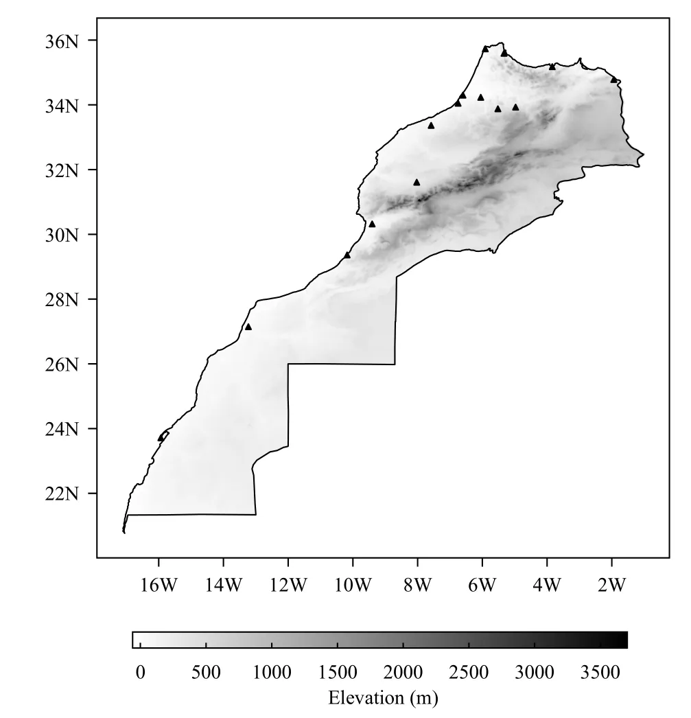
Fig. 1. Map showing orography in meters and the position of the synoptic meteorological stations used in this study, mainly located in airports, and being operational along the whole day (24 h).

3. Methods

3.1 Analog ensemble as prediction system

As shown in Fig. 2, the basic idea behind analog ensemble method is to find synonymous weather situations to the current one. To achieve this goal, we use the past forecasts database provided by a deterministic NWP model, which form analogs dataset (step 1 in Fig. 2), and a time series of analogs verifying observations, which will be ensemble members (step 2 in Fig. 2), over a given location. Taken all together, these observations constitute the ensemble prediction for the current forecast (step 3 in Fig. 2). Then, the deterministic prediction value of the predictand is the mean of the ensemble.A weather situation may extend from a few hours to a few days(weather regimes predominate the weather situation for several days). Ordinarily the forecast period of analog method is very short, often up to 6 h (Horton et al.,2017), 12 h (Riordan and Hansen, 2002), and rarely 24 h(Hansen, 2007), since analog methods often work correctly on homogeneous weather conditions which is elementary for this type of forecast. The dataset of past forecasts imperatively contains a set of meteorological variables used as predictors.

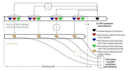
Fig. 2. Analog ensemble algorithm steps with day neighborhood and search restrictions.

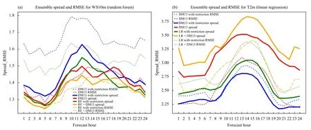
Fig. 3. (a) Dispersion diagram for 10-m wind speed (random forest) and (b) 2-m temperature (linear regression). The solid line is the average ensemble spread and the dotted/dashed lines are the root-mean-square error (RMSE) of the ensemble mean. Four configurations are shown:DM13 with all predictors weights equal to one (DM13), DM13 with weights issued from machine learning technique (RF/LR + DM13), DM13 with daily neighborhood (DM13 with restriction), and DM13 with weights issued from machine learning technique and daily neighborhood(RF/LR with restriction).

For a given location and time, one seeks to predict a variable from the set named as predictand, and uses all the eight available variables as predictors including the predictand. For example, naming the temperature at 2 m as predictand, the predictors are: T2m, RH2m, MSLP,SURFP, WS10m, WD10m, ZW10m, and MW10m from the past forecast dataset.

In order to select the potential analogs, the basic similarity metric of Delle Monache et al. (2013) has been modified and used in this study. The basic DM13 metric is defined as follows:

wheretis the current NWP deterministic forecast valid at the future timetat a station location;At′ is an analog(past forecast) at the same location and with the same forecast lead time but valid at a past timet′;Nνandwiare the number of physical variables used in the analogs search and their weights, respectively; σiis the standard deviation of the time series of past forecasts of a given variableiat the same location and forecast lead time;t? is equal to half the number of additional times over which the metric is computed; andFi,t+jandAi,t′+jare the values of the forecast and the analog in a time window withfor a given variablei.

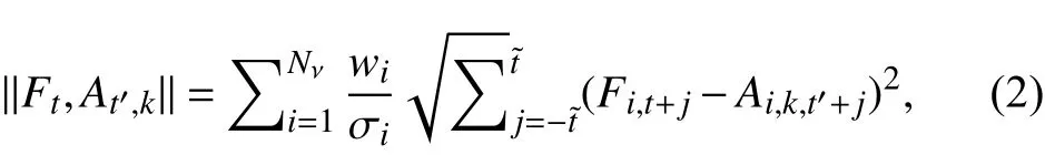
To assess the impact of the day neighboring on the AnEn performance, this criteria is added to DM13 formula in order to capture flow dependency and to force analogs to be in the same season and at a near date to the future forecast (target). Thus, Eq. (2) used in the modified version of DM13 is defined as follows:where subscriptstandt′ represent the lead times of a forecast in the future (F) and in the past (A, i.e., a potential analog) respectively. The subscriptis equal to half temporal window of additional times over which the distance is calculated; andFi,t+jandAi,k,t′+jare the values of the forecast and the analog in a time window of 2 ×h and 2 ×days for a given variablei, whereis the day window for the daily neighborhood configuration andk∈[target_date ?target_date +].

Analog search dataset (training) is restricted only to days within the day neighborhood in previous years. To retrieve the basic formula of DM13 similarity metric where AnEn looks for analogs throughout the available historical dataset, it suffices to drop daily neighborhood indexkfrom Eq. (2).

3.2 Weight optimization strategies

In contrast with the DM13 method, which uses few predictors and where predictors weights are all equal and initiated to 1, hereinstead, for every predictand from the observed features, the set of predictors is constructed from all available eight parameters. In addition, a machine learning based approach is used as a weighting strategy. Thus, three machine learning models are constructed (Table 1), tuned, and cross validated all over the training period to find the optimal weights used as input to AnEn.

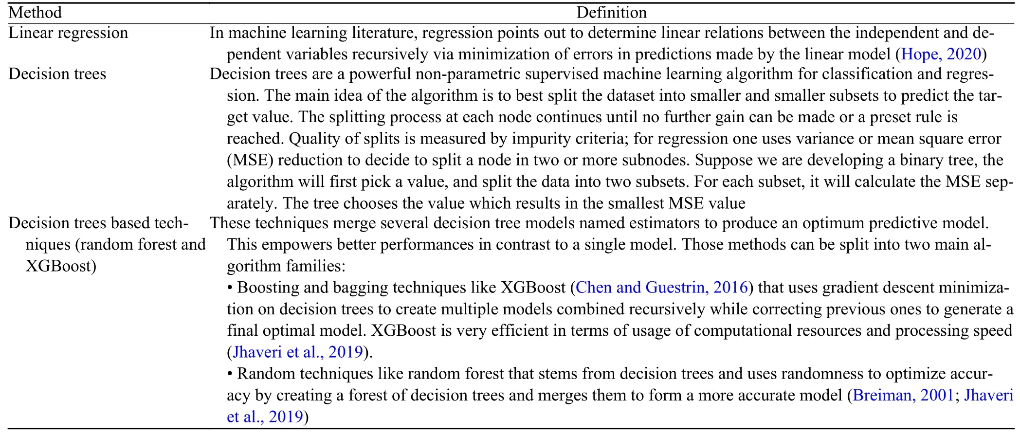
Table 1. Brief description of the machine learning techniques used for computing predictors weights

The best model found for each technique is used to find a generic equation that links the predictand to predictors (called also features), and then predictors importance’s coefficients are inferred. The importance coefficients are then scaled and normalized to form predictors weights in AnEn. Neural networks technique was excluded from the benchmark due to the hardness in physical interpretation of importance coefficients in output.Features importance is variously calculated from a machine learning techniques family to another. The minimization method is a centerpiece in the process. The ordinary least squares method is usually used to find the weights that minimize the squared differences between the actual and the estimated outcomes as in Eq. (3).

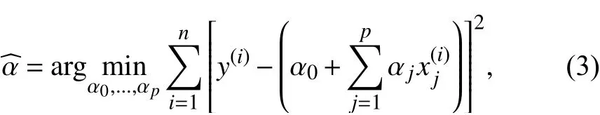
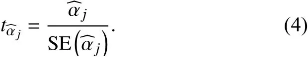
wherey(i)is theith observation for the predictandy,refers to theith value for predictorxj, and αjis the linear coefficient of predictorxj. For linear regression models predictors importance can be measured by the absolute value of itst-statistic. Thet-statisticis the estimated weightscaled with its standard error SEas shown in Eq. (4).

For the decision tree based methods, feature import-ance is defined as the decrease in node impurity times the probability of reaching that node. The node probability equals the number of samples that reach the node, divided by the total number of samples. The higher the value the more important the variable. At each split in each tree the improvement in the split criterion—here is mean square error—is the importance measure attributed to the splitting variable and is accumulated over all the trees in the trees ensemble (forest) separately for each variable.

3.3 Experimental design

For each meteorological parameter as a target predictand (T2m, RH2m, MSLP, SURFP, WS10m, WD10m,ZW10m, and MW10m), two configurations of daily neighboring are the basic DM13 version where analogs are selected from any date regardless of their season or month; and the modified version proposed in this study,where we select analogs imperatively from a day window around the day of the target. By this manner, we make sure that analogs belong to the same season as the target. This aims to assess the flow dependency of the AnEn performance, thus gaining time for operational use when looking for the best analogs.

For each configuration, a weight optimization of the eight AnEn predictors was performed over all studied airports using the three techniques (XGBoost, random forest, and linear regression), for the 1–24 forecast hours over the training period (2016–2018). For all airports, the combination leading to the lowest mean square error of the machine learning (ML)-developed model is chosen and kept constant over the testing period (2019). The set of eight predictors were used because they are considered relevant for the prediction of the target variable and are the main available parameters in SYNOP messages. This gives a potential for this to be used worldwide. Additional variables, which have not been tested in this study, could further improve the results. The DM13 basic weighting strategy is also performed and used as a benchmark.

As a result, 64 configurations (8 parameters × 2 neighborhood configurations × 4 weight optimization strategies) have been performed over all the 15 airports using the hourly AROME forecasts at the nearest grid point and the equivalent observations (Table 2). Each configuration provides a 25-member analog ensemble forecast.Allthepossiblecombinationsare defined with theconstraintwherewiisthe predictors weights. For the second category of experiments, the same configurations have been carried out, over the training period 2016–2019, to assess the impact of the boundary condition change on the AnEn performance over the testing period (2020).

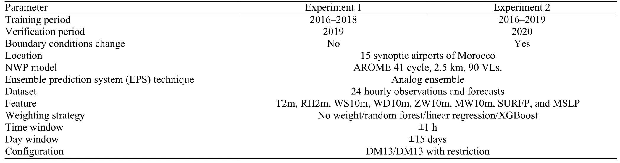
Table 2. Experimental setup with more details about the used configurations

4. Results

In this section, we analyze first the weight optimization results. Then, the AnEn’s performance with the different configurations described previously is assessed and compared to the original version of DM13 using common verification metrics for evaluation of deterministic predictions, namely Bias (mean error) and RMSE.These metrics are described with more details in Jolliffe and Stephenson (2003) and Wilks (2005). However, as an ensemble forecast, AnEn prediction system must be statistically consistent with the observations in the large scale flow given the study domain is large. This statistical consistency is assessed in this study using the spread-error diagram.

4.1 Weight optimization results analysis

Many research studies on AnEn assign equal weightswi=1to each predictor (Delle Monache et al., 2013;Delle Monache, 2015). To take into account the strength of the relationship between individual predictors and the target variable, the predictors weight optimization has been performed based on three machine learning techniques (XGBoost, random forest, and linear regression).

Table 3 shows the percentage of occurrence of all possible weight values over all airports for each predictor,where T2m is taken as predictand. It is seen clearly from this table that the past forecasted T2m is the more relevant predictor, as expected, followed by MSLP and SURFP with its weights taking values greater than 0 at 48.4% of the nearest grid points from the studied airports.

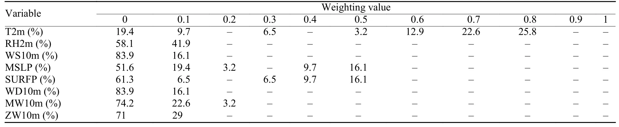
Table 3. Percentage of occurrence of possible weights values for each predictor for T2m as predictand

Results analysis for the other variables shows the relevance of MSLP and SURFP as predictors for all of them indicating the influence of large scale atmospheric conditions on each predictor. In addition, it is found that the zonal wind component also takes an important weight for RH2m as predictand. In fact, RH2m is influenced by the zonal circulation of air-masses and atmospheric flows.For zonal and meridional 10-m wind components, it is also found that 10-m wind speed is a relevant predictor.This is obvious by the nature of construction of this predictor, which is equal to the root square of the sum of wind components squares. While each variable is highly correlated with itself as predictor, some discrepancies are found between the three machine learning techniques regarding the order of high weights affectation to predictors.

Applying this static weighting strategy makes it possible to select the potential AnEn predictors for probabilistic target variable forecasting and also to find their optimal weights. This could improve the AnEn performance since their selection is based on physical link between predictors and target variables.

4.2 Statistical consistency of analog ensemble

An especially important aspect of ensemble forecasting is its capacity to yield information about the magnitude and nature of the uncertainty in a forecast. While dispersion describes the climatological range of an ensemble forecast system relative to the range of the observed outcomes, ensemble spread is used to describe the range of outcomes in a specific forecast from an ensemble system. Qualitatively, we have more confidence that the ensemble mean is close to the eventual state of the atmosphere if the dispersion of the ensemble is small.Conversely, when the ensemble members are very different from each other the future state of the atmosphere may be more uncertain (Wilks, 2005).

If on any given forecast occasion, the observationois statistically indistinguishable from any of the ensemble membersmi, then clearly the bias is zero sinceE[mi]=E[oi]. Statistical equivalence of any ensemble member and the observation further implies that

where em denotes the ensemble mean. By applying the root square to both sides of Eq. (5), it is easy to see that the left-hand side is the RMSE for the ensemble-mean forecasts, whereas the right-hand side expresses dispersion of the ensemble membersmiaround the ensemble mean (Wilks, 2005). It is important to realize that Eq. (5)holds only for forecasts from a consistent ensemble, and in particular assumes unbiasedness in the forecasts.

Two consequences of the ensemble consistency condition are that forecasts from the individual ensemble members (and therefore also the ensemble-mean forecasts) are unbiased, and that the average (over multiple forecast occasions) MSE for the ensemble-mean forecasts should be equal to the average ensemble variance(Wilks, 2005).

Figure 3 displays the dispersion diagram for 10-m wind speed and 2-m temperature. In this diagram, we have plotted the evolution of the average ensemble spread and RMSE of the ensemble mean as function of lead-time, over all the stations for both parameters. This was done for four configurations: (1) basic DM13 version, (2) DM13 with weights issued from machine learning technique and no restriction on analogs dates, (3)DM13 with daily neighborhood restriction, and (4) AnEn with daily neighborhood restriction and weights issued from machine learning technique.

For 10-m wind speed, DM13 with random forest weights and DM13 basic configurations seem to be the most statistically consistent since the spread is close enough to RMSE with the minimum RMSE linked to DM13 with random forest configuration. For T2m,DM13 with daily neighborhood restriction is the bestconfiguration in terms of statistical consistency (differences magnitude not exceeding 0.25°C) followed by AnEn configuration with daily neighborhood restriction and linear regression weights.

For the other parameters, the most statistically consistent configurations are DM13 with XGBoost weights for RH2m (difference below 1%), DM13 with random forest weights for MSLP and SURFP (difference below 0.5 hPa),and DM13 with weights from XGBoost for WD10m (not shown).

For most parameters, it is found that the good statistical consistency of the AnEn comes from a lower RMSE of the ensemble mean, which is achieved from use of higher-resolution NWP AROME model. In addition, a lower ensemble spread also contributes to the consistency of the forecast system.

Overall, it is found that configurations with weights issued from machine learning techniques without applying the daily neighborhood restriction are almost the most statistically consistent with the lowest RMSE. A more indepth assessment of a statistical consistency at a particular season or forecast lead time will be discussed later.

4.3 Deterministic verification over the study domain

4.3.1Global performance as function of lead time

In this section, the AnEn performance with the best configurations, trained during 2016–2018, is assessed and compared for each of the studied surface weather parameters over 2019, firstly to the operational NWP AROME model outputs and secondly to the AnEn configuration of DM13 where equal weights (= 1) are assigned to predictors and no daily neighborhood restriction is applied. To achieve this, Fig. 4 displays the temporal evolution of the Bias (mean error) and RMSE as function of lead time for T2m, RH2m, MSLP, SURFP,WD10, and WS10. The plotted metrics are the average value over all the 15 airports.

From Fig. 4, the performance of the operational model AROME (black line) shows a high variability, depending on the studied surface weather parameter and lead time. For instance, AROME predicts RH2m with moist bias not exceeding 3% associated with an RMSE of 10%.While AROME shows a cold bias of about ?0.5°C and an RMSE of 1.5°C for T2m. For WS10m and WD10m,AROME Bias is below 0.25 m s?1and 3 degrees respectively. For barometric fields, both MSLP and SURFP have a bias below 1 hPa and an RMSE of 2 hPa. These scores are similar to the findings of Seity et al. (2011).

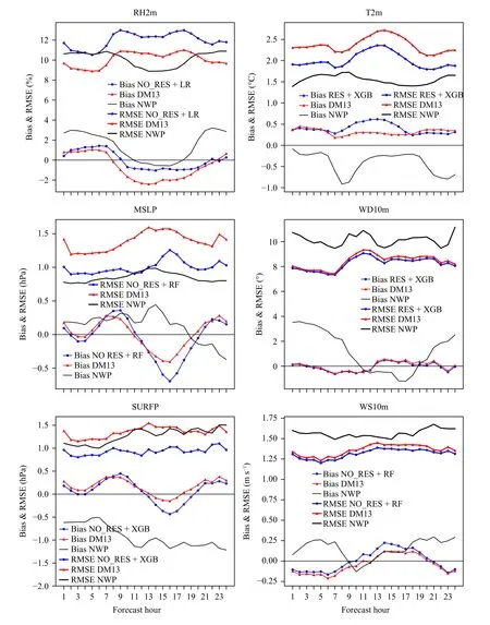
Fig. 4. Bias and RMSE curves for continuous prediction of the following surface parameters (T2m, RH2m, MSLP, SURFP, WS10m, and WD10m) using the best daily neighborhood restriction and machine learning weighting configuration (presented in dotted blue line), NWP AROME prediction of those parameters are plotted in black solid line, and finally the basic DM13 method is plotted in triangular red line.

Comparing the performances of the basic DM13 and those of the modified version configurations, the latter displays significant improvement of RMSE compared to DM13 for MSLP, SURFP, and T2m, while DM13 has the best RMSE for RH2m. Regarding the Bias, it is found that the basic DM13 has the best score for T2m,MSLP, and SURFP. The modified version shows better Bias only for RH2m; however, both methods show similar Bias values for WD10m and WS10m, where they outperform slightly each other for different lead times.

Comparing AnEn configurations and AROME performances, it is found that AnEn outperforms significantly AROME in terms of Bias during the night and early morning (lead times from 0 to 10 h and from 18 to 23 h)for all parameters. Regarding the RMSE, the best scores of AnEn are found for WS10m and WD10m.

During the nighttime forecast hours, a reduction varying between 7% and 20% of AROME’s error for WS10m, SURFP, and WD10m is perceived. These improvements in RMSE can be explained by the fact that AnEn ensemble members are constructed mainly from real observations that in 60% cases belong to the daily neighborhood (not shown), which preserves the variation in RMSE magnitude. In addition, machine learning AnEn’s configurations take into account only significant predictors. This avoids using irrelevant predictors that add more error and inaccuracy to analogs selection process. Feature selection techniques often reduce the RMSE of regression coefficients, in particular for weak or noisy predictors (Heinze et al., 2018). However, a slight degradation of the RMSE is found for the thermodynamic surface parameters (RH2m and T2m) in comparison with AROME (Fig. 4). This could be due to the high spatiotemporal variability of these parameters and also to the model forecast error. This might indicate that AnEn needs more predictors representing the lower layer of the atmospheric boundary layer instead of using only the main surface weather parameters issued from the SYNOP messages.

From a seasonal dependency point of view, it is found that the modified version AnEn DM13 yield improvement of Bias and RMSE in winter and spring during the daytime forecast hours (from 10 to 18 h) while slight worsenings are found for both metrics in summer and autumn (not shown). This is mainly due to the limited ability of AROME in predicting the rapid convective mesoscale situations during these months (Seity et al., 2011).In the next section, the spatial distribution of AnEn performance is investigated to assess any dependency of region and season.

4.3.2Global performance as function of spatial location

To assess the global performance of AnEn over the study domain, the Bias and RMSE gain/loss [Eq. (6)], in comparison with AROME, have been calculated for each airport over all the lead times and are plotted spatially(RH2m as an example in Fig. 5) for DM13 and the best configuration of the modified version of DM13.

where Scoreanenand Scorenwpare relatively the scores for AnEn and NWP.

Indeed, when the NWP score is perfect (= 0), this score is converted to 0.01 to avoid infinite loss value.

For 2-m relative humidity (Fig. 5), AROME model draws a positive bias over coastal areas (up to 10%), and negative bias for two airports in the northeastern part,while the RH2m bias is very weak in the other airports.With regard to AROME, AnEn yielded an important improvement by reducing RH2m Bias by up to 50% for almost all the airports while it reduced the RH2m RMSE by about 25%. It should be noted that AnEn degrades the AROME Bias in six airports in the north part of Morocco; most of these stations already have an almost perfect Bias by AROME.

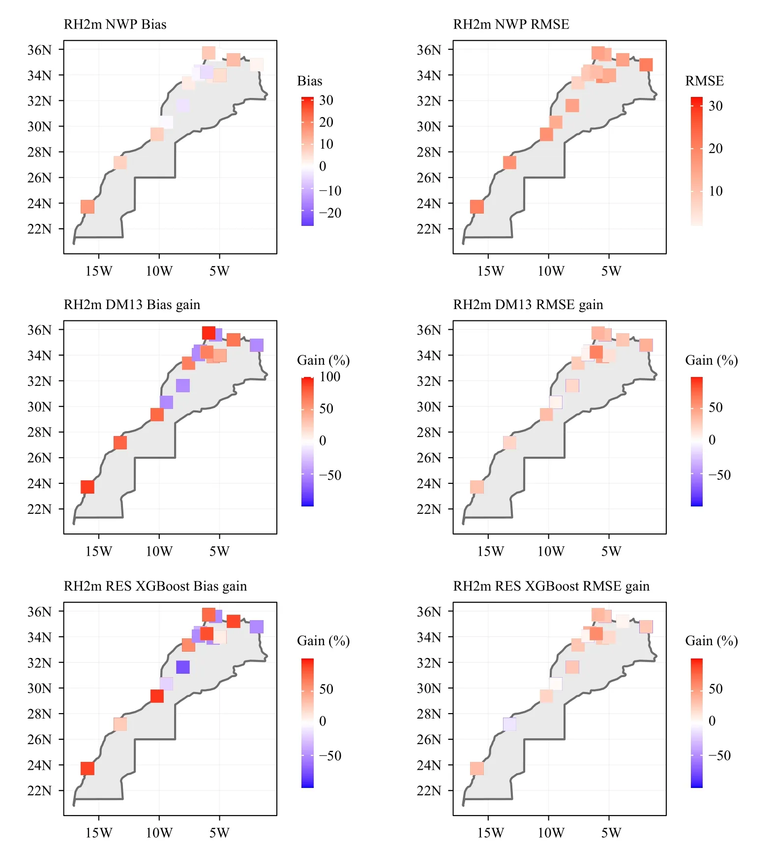
Fig. 5. Bias and RMSE gain of RH2m at each airport for DM13 and AnEn’s best configuration. The same metrics (Bias and RMSE) for the operational AROME NWP model at each station are also plotted as a benchmark.

Similarly, the spatial AnEn performance analysis for the other surface parameters points out that AROME shows a negative Bias for T2m especially over coastal areas (not shown), while AnEn highlights an improvement up to 50% in Bias and 25% in RMSE for most of the airports from different regions (Mediterranean, Atlantic coastal areas, southern region, interior, and eastern region). For the rest of airports, AnEn converts negative Bias to positive Bias with magnitude not exceeding 1.5°C.

Besides, AROME highlights a negative bias for mean sea level pressure and surface pressure all over Mediterranean and Atlantic coastal areas and a weak bias far inland. AnEn reduced pressure bias and RMSE magnitude concurrently by 50% for most airports, except a few interior airports where AnEn degrades these metrics. AnEn best configuration reduced Bias and RMSE of wind speed by more than 40% of its magnitude, this finding is generalized for all airports.

For wind direction, AROME underlines very weak Bias in general except for few interior airports where Bias exceeds 9 degrees, while AnEn reduced Bias magnitude in those areas to 2.5 degree or by 50% and preserved slightly bias nullity all over the rest. The RMSE of wind direction was reduced by AnEn up to 60%. For wind components, AROME represents a negative Bias over all airports (range from ?20 to ?5 m s?1), AnEn lower Bias magnitude by 70%. In addition, RMSE error was reduced by 75% for 10-m wind components.

In Figs. 6 and 7, we have plotted the seasonal spatial distribution of gain/loss in Bias and RMSE for T2m, using DM13 random forest configuration. It is seen clearly that AnEn performances are seasonally dependent. Indeed, Bias gain exceeds 50% for most of the airports especially in autumn and summer; while a general worsening is found in spring, one can remark that Bias gain reached 70% for some locations on the Atlantic side. Regarding the RMSE, seasonal gain for T2m is around 20% for at least half of the studied airports except for spring.

Overall, the gain/loss behavior for Bias and RMSE is different from one parameter to another and is highly dependent on season and location. In this context, Bias gain exceeds 50% for 70% of parameters (not shown). Slight degradations are observed in the airports with good seasonal Bias.

A limitation of AnEn is a slight degradation of seasonal RMSE for some tested configurations and parameters(not shown). This RMSE loss is mainly observed in the Mediterranean and eastern airports (Tanger, Al Hoceima,and Oujda). It is also found that neighborhood restrictions showed valuable improvements for some parameters (T2m, RH2m, WS10m) and contributed to increase the RMSE and Bias gain for different locations and seasons for those parameters.

4.4 Sensitivity to boundary conditions

As mentioned before, AnEn leverages a single deterministic NWP model to produce probabilistic forecasts.Thus, it is highly recommended to use the same model.In our case, only the lateral boundary conditions have been changed in 2020.

First, the impact of this change on the AROME performance itself is assessed. It is found that the new boundary condition coupling used in 2020 softly impacted AROME’s performance for most of the parameters (10-m wind speed is shown as an example in Fig. 8).Indeed, improvements in RMSE (not shown) and Bias are noticeable mainly for synoptic dynamical parameters such as MSLP, SURFP, WS10m, and 10-m wind components. On the other hand, AROME’s performances are of no significant change for RH2m, T2m, and WD10m.

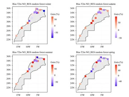
Fig. 6. Bias gain/loss for T2m for all seasons using no daily neighborhood restriction and random forest weights configuration.

Fig. 7. RMSE gain/loss for T2m for all seasons using no daily neighborhood restriction and random forest weights configuration.

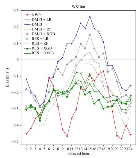
Fig. 8. Wind speed Bias over 2020 for all lead times and all the possible AnEn configurations.

However, AnEn performance was not affected by the boundary conditions change. Indeed AnEn still outperforms AROME spatially, temporally, and seasonally for most of the surface parameters and locations. AnEn still shows best Bias and RMSE during nights and mornings over 2020 for most of the surface parameters. A finding to underline is that AnEn Bias gets improved during day lead times where it overtakes AROME for all parameters except MSLP and SURFP. On the other hand, AnEn RMSE remains the best overall. It is to mention that AnEn best configurations of 2019 are not preserved for 2020. For instance for WS10m, the best AnEn configuration during 2019 was DM13 + RF while it is DM13 +XGB for 2020.

5. Discussion

In this study, it is demonstrated that the best configurations with multiple criteria of AnEn yield important improvement in surface weather parameters forecasting but it still has some shortcomings.

Indeed, the perfect analogy is far from existing, but identifying close enough situations leading to similar effects is still possible. Then, the relevance of analogy and thus analogs forecasting quality is tightly affected by the three major following factors: i) the process of skillful analogs selection in the training data, which depend on the similarity metric, predictors weighting and selection,temporal window around the target lead time, and the number of members; ii) the target surface weather parameter and its predictability by data-driven forecasting techniques; and iii) the used NWP model error in the training data and its ability to forecast rare events and some mesoscale phenomena (Zhao and Giannakis, 2016).

In this research, we tackled the main surface weather parameters issued from SYNOP messages. While AnEn improves the synoptic scale parameter forecasting(MSLP, SURFP, WS10, and WD10) by reducing both Bias and RMSE, it is found that AnEn improves slightly the Bias but degrades the RMSE for the thermodynamic surface parameters (RH2m and T2m) during the daytime lead times and also spatially in some airports. This could be overcome by adding predictors representing the lower layer of the atmospheric boundary layer in addition to parameters that describe the atmospheric circulation such as geopotential fields in many levels (Duband, 1981;Guilbaud, 1997) or new sets of predictors at different pressure levels (Z500, TPW850, etc.) (Horton et al.,2012). In fact, even for two locations that are close to each other but subject to different critical atmospheric conditions, the selection of the best predictors can vary.Thus, the method needs to be adapted to local conditions,available data, and the size of the region of interest. In this framework, three machine learning techniques (linear regression, random forest, and extreme gradient boosting) have been used in this study to find the optimal weights for the physically meaningful predictors. This step of AnEn forecasting process aims to maximize the useful information and reduce noise. The optimal importance of predictors however varies from region to another,a season to another, and along with the leading atmospheric process. Indeed, Junk et al. (2015) stated that optimized predictor weights are highly affected by terrain complexity and atmospheric stratification. In our case,using machine learning technique to optimize the predictor weights leads to an improvement in Bias and RMSE exceeding 50% while the gain reached 21% in Gensler et al. (2016), 20% in Junk et al. (2015), and 44% in Wang et al. (2019).

One key aspect in the analogy is the seasonal preselection of the analogs. This preselection is implemented in this study as a moving selection of ±15 days centered around the target date for every year of the archive and time window of ±1 h around the forecast hour since the hourly forecasts are used here and are issued from a high-resolution mesoscale operational model. However,it is found that seasonal preselection yields worsening of AnEn performance in some airports. Indeed, for one target day, the sampling (31 days/yr × 3 yr of training = 93 days) might be inadequate to retrieve the skillful analogs due to the missing observed values or to the occurrence of rare events in this temporal window. Thus, it is concluded that this approach requires a very long archive that is why no restriction on target date neighboring performs better. Indeed, an analysis of the selected analogs position from the target has been performed and it is found that for some cases, many analogs get outside the daily neighborhood window (±15 days). Hence, it would be very beneficial to extend that window. This is in line with the finding of many previous studies for climate purpose that uses daily neighborhood criterion to detect relevant analogs (Bontron, 2004; Horton et al., 2012; Ben Daoud et al., 2016). In ensemble forecasting, the number of members is a parameter of higher relevance. Hence,finding the optimal number of members (analogs) that improves AnEn performances is highly demanded (Horton, 2019; Li et al., 2020). Furthermore, beyond topography, a more precise distinction between spatial areas(urban and non urban for example) can enhance AnEn performance interpretation and point out the ability of using such methods in highly dense urban cities (Li et al.,2020). In addition, some research studies used a large forecast range to investigate the potential of AnEn to capture well the diurnal cycle of the weather surface parameters such as T2m and WS10m (Wang et al.,2019).

6. Conclusions

This study presents a new application of the analog ensemble method to improve surface weather parameters prediction over 15 airports of Morocco during 5-yr period (2016–2020), from the non-hydrostatic mesoscale operational model AROME hourly forecasts and observations issued of SYNOP messages. The analog ensemble method application is extended for the first time to include eight main weather surface parameters (T2m,RH2m, MSLP, SURFP, WS10m, WD10m, ZW10m, and MW10m). Seasonal impact was considered in the analogs search process by applying daily neighborhood restriction, in a way that all the analogs have the same season as the current forecast. Best analogs for AnEn are searched by using the studied parameters as predictors,given optimized weights that are calculated as a normalized feature importance coefficients issued from machine learning techniques (linear regression, random forest, and XGBoost) over the training period(2015–2018). Verification of the performance of AnEn was carried out mainly over 2019. An additional verification over 2020 also was held to assess AnEn sensitivity to lateral boundary conditions change.

The results from the spatial and temporal scores analysis showed that AnEn best configurations produce notably lower Bias and RMSE compared to AROME during night lead times, especially for large scale synoptic parameters (SURFP, MSLP, WD10m, and WS10m).However during day lead times, AnEn shows some limitations, in particular for thermodynamic surface parameters (T2m and RH2m). This is mainly due to the high spatiotemporal variability of these parameters and also to the high RMSE of the ensemble mean and also to higher ensemble spread in some cases during daytime hours. Similar results are reached by AnEn also for most airports,indicated by spatially averaged Bias and RMSE reduction up to 50% and 30% depending on the season. Despite the advantage of lower computational cost, seasonal preselection yields a performance degradation in some airports almost due to the weakness of sampling adequacy.

According to World Meteorological Organization(WMO), the wind speed value is rounded to the nearest integer in the SYNOP messages. Then, the accuracy of the wind measurement is 1 m s?1. Similarly, the wind direction is coded in a wind rose with 36 directions. This induces an uncertainty of about 10 degrees. The 2-m relative humidity is also rounded to the nearest integer. Consequently, this leads to an accuracy of 1%. All these observation error sources impact the assessment of the AnEn performance while using the continuous verification scores such as Bias and RMSE. One way to overcome these limitations is using the precise observed values from the automatic weather stations that have become an increasingly prominent part of meteorological observation networks over the last 20–30 years and most or all synoptic observations are now automated in some countries.

The results reported herein can be further improved with a longer training dataset, by extending existing training datasets to consider neighboring locations while searching analogs, exploring further similarity metrics,and by adding more predictors from lower layers of the atmospheric boundary layer or parameters that describe the atmospheric circulation predictors.

Acknowledgments.We would like to thank reviewers for taking the time and effort necessary to review the manuscript. We sincerely appreciate all valuable comments and suggestions, which helped us to improve the quality of the manuscript.