FEQ: a new flux coordinates based equilibrium solver including both magnetic axis and separatrix

Xinhao JIANG (蔣鑫浩) and Youwen SUN (孫有文)

1 Institute of Plasma Physics,HFIPS,Chinese Academy of Sciences,PO Box 1126,Hefei 230031,People's Republic of China

2 University of Science and Technology of China, Hefei 230026, People's Republic of China

Abstract Accurate tokamak plasma equilibrium solution in flux coordinates is crucial for many stability and transport studies.Different approaches for dealing with singularities in solving the nonlinear Grad–Shafranov (GS) equation in flux coordinates or also known as straight field line coordinates are proposed in this paper.The GS equation is solved by iterating the position of grids directly in flux coordinates,and hence,no additional errors are introduced due to mapping process for a convergent solution.The singularity at magnetic axis in flux coordinates is removed by using a novel coordinate transform technique.Different from other techniques previously developed,no assumption in boundary condition at magnetic axis is used.This is consistent with the fact that there is no physical boundary at the magnetic axis.A flux coordinate system with poloidal coordinate chosen as the geometric poloidal angle is proposed.It conquers the difficulty in no definition of poloidal coordinate in flux coordinates at separatrix because of the singularity at x-point(s)in a divertor configuration.It also simplifies the process for computing poloidal flux coordinate during the iteration for solving the nonlinear GS equation.Non-uniform grids can be applied in both radial and poloidal coordinates,which allows it to increase the spacial resolution near x-point(s) in a divertor configuration.Based on the model proposed in this paper, a new Flux coordinates based EQuilibrium solver (FEQ) in tokamaks is developed.The numerical solutions from this code agree well with both the analytic Solov’ev solution and the numerical one from the EFIT code for a divertor configuration in the EAST tokamak.This code can be applied for simulating different equilibria with prescribed shape, pressure and current profiles,i.e.including both limiter and divertor configurations, positive triangularity and negative triangularity, different β, arbitrary magnetic shear profile etc.It provides a powerful and convenient fixed-boundary inverse equilibrium solver including both magnetic axis and separatrix in the solution for tokamak researches.

Keywords: equilibrium, flux coordinates, tokamak

1.Introduction

MHD equilibrium plays a crucial role in nuclear fusion studies.It is the basis of almost all of the fusion researches,such as plasma stability, transport, radio-frequency waves for heating and current drive etc [1–6].In a tokamak, because of the toroidal symmetry, the MHD equilibrium equation is reduced to the so-called Grad–Shafranov(GS)equation[7,8].It is a nonlinear equation, which is often solved numerically for a general equilibrium configuration.Many numerical codes have been developed in the past.They can be roughly divided into the following categories:finite difference method[9], finite element method [10], conformal mapping method[11] and Green’s function method [12] etc.For experimental applications, the EFIT code [12] is broadly used to reconstruct the plasma equilibrium using magnetic measurements as well as kinetic profiles in many tokamaks.

In plasma stability and transport studies etc [1–6], it is often convenient to employ flux coordinates for a given plasma equilibrium.In this paper, the flux coordinates specifically refers to straight field line coordinates [13, 14].A mapping process from the real space coordinates to the flux coordinates is often necessary, if the equilibrium solution defined on real space coordinates provided for example by the EFIT code [12].In this process, one has to employ twodimensional interpolation and numerical integration along the contours of flux surfaces,which may produce truncation error and reduce the accuracy of the original equilibrium especially near the plasma core.Therefore, an accurate equilibrium solver based on flux coordinates also known as inverse equilibrium solver is required.

Some inverse equilibrium solvers [15–19] have been developed in the past.Inverse equilibrium solvers can generally be divided into three categories [20], i.e.the iterative metrics method[15,18,19],the direct solution of the inverse equilibrium equation [17] and expansion in poloidal angle method[16].For inverse equilibrium solvers,it is known that there are some challenges in the numerical issues on singularities.Due to the choice of flux coordinates,GS equation is singular at the magnetic axis.An approximate method using a boundary condition was often used to deal with the singularity near magnetic axis [15].However, there is no physical boundary at the magnetic axis.

Divertor configuration with separatrix is also a challenge for inverse equilibrium solvers.There is no definition of the usual flux coordinates on the separatrix because of the singularity at x-point.Therefore,the x-point is often removed by smoothing the separatrix positions like that used in the CHEASE code [10].It is just an approximate method for dealing with separatrix.Another approach is to define the Jacobian matrix in terms of grid element geometry and to make the stability functional approximately invariant with respect to the poloidal coordinate[21,22].Recently,a newly developed EEC code [19] employing Hermite elements has been capable to deal with the separatrix in modeling of edge plasma equilibrium with a method of coordinate transformation.To get full plasma equilibrium, it needs to be combined with an equilibrium solver ESC [23] for the plasma core.

In this paper,we propose different approaches for dealing with those singularities to include both magnetic axis and separatrix in the solution of GS equation and employ the finite difference method with nonuniform grids, based on which a new fixed-boundary Flux coordinates based EQuilibrium solver(FEQ)in tokamaks is developed.The numerical model and the implementation of FEQ are presented in section 2,the new methods for dealing with singularities are presented in section 3,and benchmarks of the FEQ code with the analytic Solov’ev solution and the EFIT code are presented in section 4.Some applications of this code for modeling of different types of tokamak plasma equilibrium are shown in section 5, followed by a summary and conclusions in section 6.

2.Numerical model of the FEQ code

2.1.GS equation in flux coordinates

The well known GS equation [7, 8] can be written as

where ψpis poloidal magnetic flux (normalized to –2π),p=p(ψp) is pressure profile, g=g(ψp)=RBTand BTis toroidal magnetic field.Here Δ*is a two-dimensional secondorder differential operator.In flux coordinates (ρ(ψp),θ,ζ),it can be written as

Here ζ ≡φ ?qδ is a toroidal like angle, φ is the geometric toroidal angle, q=q(ψp) is the safety factor profile, and δ=δ(ψp, θ) is a periodic function on each flux surface.Because of toroidal symmetry, it does not appear in the equation.More detailed information about flux coordinates and different form of GS equation can be found in appendices A and B, respectively.

GS equation can be solved with prescribed the radial profiles of p(ψp) and g(ψp), and plasma boundary shape together with a boundary condition.

2.2.Iteration for solving the nonlinear GS equation

We employ a Picard iteration method similar to that used in the EFIT code [12] to solve the nonlinear GS equation.Different from the EFIT code that the poloidal magnetic flux is calculated in the real space, FEQ is updating the positions of grids in the real space[ ]R Z, for given grids in flux coordinates (ρ, θ) during the iteration process.With an initial guess ofand the grids( )=R Z,k0,the grid positions(R,Z)k+1are updated by searching the positions of new flux surfaces determined by the solution of(ρ,θ)kon the grids (ρ, θ) at the kth step, which can be solved from the matrix form of GS equation

together with a fixed outer boundary condition

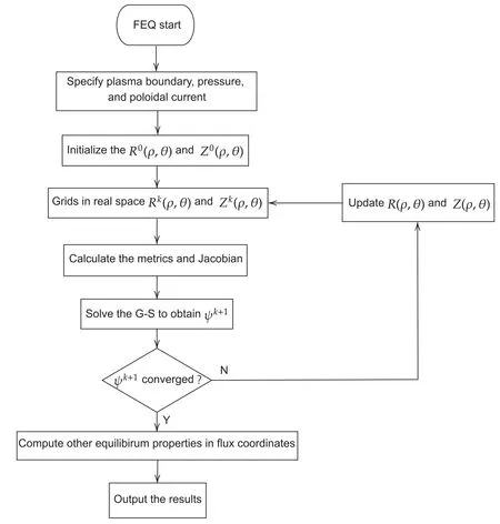
Figure 1.Flowchart of the FEQ code.

Equation (3) is directly solved by using the backslash operator in Matlab at each iteration [24].In most cases, a simple way for initial guess can be applied.The magnetic axis(R0,Z0)is chosen at the center of given plasma boundary.The normalized poloidal flux is chosen as=ρ2=r?2, where[ ]∈0, 1 is the normalized minor radius at each poloidal angle.It means that the initial grids(R,Z)k=0are chosen as evenly distributed inside the boundary, i.e.R=R0+

A flowchart for this process described above is summarized and shown in figure 1.After the solution is converged to a prescribed tolerance of error,other equilibrium quantities such as q profile,magnetic shear,curvature etc required for stability and transport studies will be evaluated.Equations for calculating Jacobian and the metrics related to ρ and θ of the flux coordinates are listed in appendix B.Some detailed information of numerical techniques on searching magnetic axis and new flux surfaces etc can be found in appendix C.

2.3.Finite difference method for solving the GS equation

In this work,finite difference method[24,25]is employed to construct.For a one-dimensional function f(x), as long as differentiable, the finite difference form of the mth derivative of f atcan be written as

where and the number of points n in the stencils determines the order of accuracy in the difference approximation.Herecan be evaluated using the routine described in the reference.It supports non-uniform grids of →and is adjustable to arbitrary prescribed orders of accuracy by changing number of points in the stencils[24].In this we only used the second-order accuracy of finite difference form.

The matrix form of the two-dimensional differential operatorscan be constructed based on the one-dimensional form in equation(5).In this convention,is a sparse banded tridiagonal matrix.

3.New methods for dealing with singularities in flux coordinates

3.1.Dealing with singularity at the magnetic axis

Let introduce a local orthogonal coordinate system (x, y)in real space

It is just a shift of origin to the magnetic axis and then a rotating of the coordinates (R, Z) with a poloidal angle θ0as shown in figure 2.To link the derivatives between flux coordinates and(R,Z)coordinates,additional local coordinate system (u, v) is introduced with their definitions

They are aligned with the x and y coordinates, respectively.As shown in figure 2, it is just a connection of radial flux coordinates at opposite poloidal angles.

The differential operator at the magnetic axis is defined in this new coordinate system (u, v), which can avoid the singularity in the flux coordinates.It can be expressed as

3.2.A flux coordinate system making the computational domain covering both magnetic axis and separatrix

As shown in appendix A,there is a freedom in the choice of θ to construct a flux coordinate system.We propose to use a flux coordinate system by choosing θ=θg, where θgis the well defined geometric poloidal angle.The flux coordinate system is usually singular at the magnetic axis and the separatrix for a divertor configuration.However, the poloidal coordinate can still be well defined at these singular surfaces in this flux coordinates.Therefore,the two-dimensional grids of this flux coordinates (ρ, θ) are well defined covering both magnetic axis and separatrix.It is also obviously convenient for the modeling of equilibrium here.There is no necessary to do surface integration for constructing θ during the iteration.

Figure 2.Magnetic surface in real space and the points that we pick to represent the partial derivatives at the magnetic axis.

Because the separatrix appears as boundary condition in the equilibrium problem, there is no singularity in the matrixusing finite difference method.The only issue is that the spacial resolution near the x-point is not so good.This can be solved by using a non-uniform grids.

Our choice of the straight magnetic field line flux coordinates is(θ,ζ=φ ?qδ)for a specified angle θ[1].There are different ways in choosing the radial coordinate ρ.It is in principle can be chosen as any flux surface function.In this work, we chose

As shown in appendix A, the choice of θ=θgis equivalent to choose

where l is the arc length of the field line in the poloidal plane.

To construct a flux coordinates as described in appendix A,the left task is to evaluate the toroidal shift qδ for ζ, which can be integrated along the field line in poloidal plane from

Equation (11) is singular at the separatrix.However, for the application of flux coordinates, qδ mainly contributes to make field aligned for accurate evaluation of the parallel derivative [26].Therefore, the real singularity is at the xpoint, where Bp=0, but not the whole separatrix.Since the toroidal coordinate is often ignorable because of toroidal symmetry, the singularity in other equilibrium quantities can be avoided in many applications, which is beyond the scope of this paper.Although the ζ coordinate does not enter the GS equation because of toroidal symmetry, the choice of this coordinate might be useful for future application on stability studies as discussed in appendix A.

Figure 3.(a) Comparison of magnetic flux surfaces between the FEQ simulation result (red dashed line) and the analytic Solov’ev solution(blue solid line) with q0=0.75, κ=1, R0=1 and a=0.5 in equation (14).(b) Evolution of maximal convergience error compared toprevious iteration.(c)Evolution of maximal error compared to the analytic Solov’ev solution using uniform(red line with crosses)and nonuniform (blue line with pluses) grids.

Please note that any flux coordinates including the one used here are singular at magnetic axis and x-point.If a stability code needs to evaluate all of the flux coordinates (ρ, θ,ζ),one may has to exclude the magnetic axis and smooth the last closed flux surface near the x-point similar to the method that used in the CHEASE code[10].Therefore,the option for smoothing the last closed flux surface is also included in the FEQ code.

4.Benchmark and illustration of capability for modeling divertor configuration

4.1.Benchmark with the analytic Solov’ev equilibrium solution

For code validation,we at first compare the numerical results to an Solov’ev equilibrium solution for constant profiles of[27].Choosing

the analytic equilibrium solution of poloidal magnetic flux ψpcan be written as

Here q0is the safety factor on the magnetic axis, κ is elongation, R0and a are major and minor radius, respectively.

Figure 3 shows a comparison of magnetic flux surfaces between the FEQ result and the analytic Solov’ev solution with q0=0.75, κ=1, R0=1 and a=0.5 in equation (14).Using a mesh of 51×257 and packing slightly the radial grids near the plasma boundary and the poloidal grids near 2π/3 and 4π/3 as shown in figure 3(a), the analytical results(blue solid lines) can be accurately reproduced by the FEQ simulation results (red dashed lines).The maximal absolute error of the FEQ simulation result compared to the analytic solution is less than 8×10?5after 5 iterations(blue line with pluses) as shown in figure 3(c).The convergence error of radial force balance can be easily controlled to be much lower than this value.For comparison, the result using a uniform grids (red line with crosses) is also shown in figure 3(c).In this study, we used the grid mapping method described in chapter 2 in [25] for grid packing.In the uniform grids case with same number of grids, the maximal error is about 3×10?4.This shows the advantage of the non-uniform grids.

Figure 4.Dependence of the maximal absolute error in the numerical solution on grid density with uniform gird(orange line with crosses)and non-uniform grid(blue line with pluses)respectively,compared to a third order accuracy reference (red dashed line).

Figure 5.(a)Comparison of magnetic flux surfaces between the FEQ simulation result(red dashed line)and the analytic solution(blue solid line)with an x-point at the boundary.(b)Dependence of the maximal absolute error in the numerical solution on grid density(blue line with pluses), compared to a third order accuracy reference (red dashed line).

We have performed a scan of grid density to check the maximal absolute error dependence for both uniform grids(orange line with crosses) and non-uniform grids (blue line with pluses) cases as shown in figure 4.The advantage of non-uniform grids can be found clearly especially in the less dense grid cases.It is shown that the achieved accuracy is around third-order, which is better than the expected secondorder accuracy using a 3-points finite difference form.This may be partially benefited from the improved accuracy in the step for updating grid positions using interpolating.

4.2.Benchmark with an analytic equilibrium solution with an x-point at the boundary

To demonstrate the capability of modeling divertor plasma equilibrium configuration,an analytic solution with an x-point at the boundary is used for another benchmark in this section.

The analytic equilibrium with an x-point at the boundary can be constructed by adding some upper-lower asymmetric polynomial homogeneous solutions [28] into the Solov’ev equilibrium solution in equation (14).For example, a term ψx=(3R2?4Z2)R2Z is used in [19] to generate analytic equilibrium with an x-point at the plasma boundary.For simplicity,we employ the same form of analytic solution that used in [19]

Figure 5(a) shows another comparison of magnetic flux surfaces between the FEQ simulation result and an analytic equilibrium solution with R1=5, R2=7, Z2=4.5, A=–0.0005,B=0.01 in equation(15).This analytic solution has a strong shaping and a lower single x-point at the plasma boundary.The analytical results(blue solid lines)can be well reproduced by the FEQ simulation results (red dashed lines).Dependence of the maximal absolute error in the numerical solution on grid density (blue line with pluses) is shown in figure 5(b).Similar to the case in figure 4, the achieved accuracy is again around third-order (red dashed line), which is better than the expected second-order accuracy using a 3-points finite difference form.This demonstrates the capability of the FEQ code for modeling tokamak plasma equilibrium with an x-point at the boundary.

4.3.Modeling of divertor equilibrium configuration using the EFIT output

Figure 6.Comparison the poloidal magnetic flux (a) and q (c)between the outputs from the EFIT reconstruction (blue solid line)and the FEQ outputs(red danshide line)using the inputs for plasmaboundary and the(b)two kinetic profiles ? from the EFI T outputs of an equilibrium in EAST discharge 52 340.

Figure 7.Comparision of the very edge magnetic flux surfaces at ψp=0.9000, 0.9167, 0.9333, 0.9500, 0.9667, 0.9833, 1.0000 from the EFIT(blue solid line)and the FEQ (red dashed line)outputs for the same equilibrium as that in figure 6.

In order to verify the performance of FEQ in the application for the simulating experimental results,an equilibrium with a mesh 129×129 in the [R, Z] coordinates for a single null divertor configuration in an H-mode discharge 52 340 in EAST reconstructed from the kinetic-EFIT code [29] is used as an input for the FEQ code.

Figure 8.Example equilibrium with negative triangularity δ=–0.5.

Using a mesh of 51×129 and packing the radial grids near the plasma boundary and the poloidal grids near the x-point, the convergence error is less than 10?5after 32 iterations,which takes around 155 using a PC with a 2.3 GHz CPU.Figure 6 shows a comparison between the EFIT reconstruction results and the numerical results simulated by the FEQ code using the inputs for plasma boundary and the two kinetic profilesfrom the EFIT outputs.It is shown that the simulated distribution of the flux surfaces(red dashed dotted line) agrees well with the EFIT output (blue solid line)as shown in figure 6(a).The used inputs about the two kinetic profiles are shown in figure 6(b).The q profile simulated by the FEQ code also agrees well with the EFIT output as shown in figure 6(c).The spacial resolution near the plasma core is much improved in the FEQ code results because of using flux coordinates compared to the EFIT outputs defined in real space.This guarantees for accurate modeling of plasma stabilities near the plasma core.

Figure 7 shows a detailed comparison of the edge magnetic surfaces near the x-point.It shows that the separatrix can be included in the solution and the results agrees well with the EFIT output.This provides accurate equilibrium near the plasma edge, which is essential for edge stability studies.

In this kind of simulation, the direct mapping flux surfaces from the outputs of EFIT [14] can also be used as an initial condition to speed up(around 50 s or 13 iterations)the convergence of the FEQ code.For an realistic equilibrium like the one used in figure 6, a reasonable accurate equilibrium can be simulated within one minute, which is fast enough for many applications.

5.Examples for applications

5.1.Negative triangularity configuration case

Recently, it is found in both experiments and modelings that negative triangularity configuration has attractive advantages over the positive ones for plasma stability and confinement[30].The FEQ code can be applied for arbitrary prescribed plasma boundary.Therefore, it can be easily applied for simulating plasma equilibrium with different shapes.In order to show the high practicability of FEQ, a case of negative triangularity divertor configuration was simulated as shown in figure 8.The boundary is just a horizontal flip of the experimental one in the EAST discharge 52 340 shown above.It is also a divertor configuration with a lower single null.It is easy to see in figure 8(a) that the application of non-uniform grids can reduce the number of grids to describe the sharp shaping of the flux surfaces near the x-point.This demonstrates the capability in modeling plasma equilibrium with different shaping.

Figure 9.High βp equilibrium with βp=4.01 for circular plasma boundary.

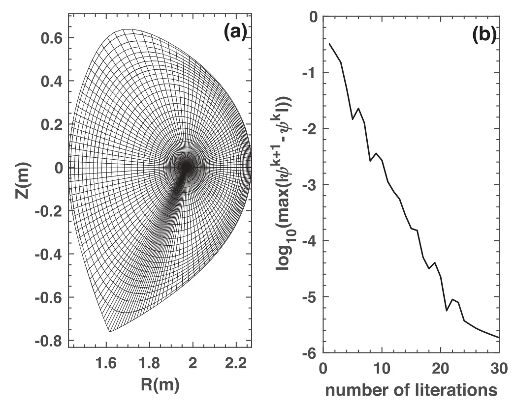
Figure 10.Scaled high βp equilibrium with βp=4.12 using the plasma boundary in figure 6.

5.2.High βp equilibrium

High βpscenario in tokamaks can generate high fraction of bootstrap current, which is necessary for sustaining steady state operation in a fusion reactor.However, the high-β equilibrium with a large Shafranov shift is challenging for some inverse solvers[23].FEQ is also quite effective in simulating high-βpequilibrium.Two examples for limiter and divertor configurations are shown in figures 9 and 10, respectively.Significant Shafranov shift can be found in both of these two cases.From the example of circular configuration, the magnetic axis is greatly shifted to the low field side under the high-βpconfiguration.Figure 10 shows a high-βpequilibrium constructed from the plasma boundary of the EAST discharge 52 340 used in previous section.The result demonstrates that the FEQ code can also be very effective for simulating high-βpequilibrium with a separatrix.

Lastly, the non-uniform grids capability in both radial and poloidal directions allow us refining the grids at any position we are interested.It is especially important to refine the grids near the rational surfaces for the stability analysis for realistic low resistivity.It is also important for a divertor configuration to refine the grids near the x-point as shown in figures 8 and 10.This shows a great advantage of the FEQ code.All of the results presented above demonstrate the robustness and high capability of the FEQ code.

5.3.Construction of flux coordinates for future application

The construction method of the flux coordinates is introduced in appendix A.FEQ is based on the flux coordinates proposed in this paper.Different from other flux coordinates, the poloidal coordinate is a direct output.It is only necessary to compute the toroidal shift qδ to get ζ.Please note again any flux coordinates cannot be defined at magnetic axis and xpoint.Figure 11 show one example of the two-dimensional(a) and three-dimensional (b) views of the grids in this flux coordinates.Based on the solution in this flux coordinates, it is also easy to transform it to any other flux coordinates as described in appendix A.For example, the same distribution of grids in Hamada result is shown in figure 12.

The accuracy of radial force balance can be well controlled on all of the grids with an prescribed error of tolerance and no interpolation is necessary for the following studies.Different from the equilibrium code based on the coordinates in real space and some other inverse equilibrium solvers, it can provide equilibrium solution with high accuracy on all of the flux surfaces including both magnetic axis and separatrix,which is necessary for many stability and transport studies.

6.Summary and conclusions

Figure 11.Two-dimensional (a) and three-dimensional (b) views of the grids in the flux coordinates with poloidal coordinate chosen as the geometric one.

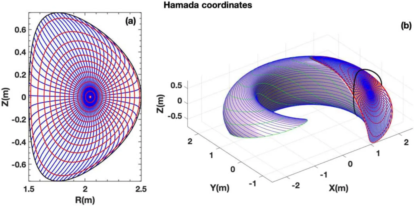
Figure 12.Two-dimensional (a) and three-dimensional (b) views of the grids in the Hamada coordinates.

In summary, a new inverse tokamak plasma equilibrium solver FEQ is developed.It can provide accurate tokamak plasma equilibrium solution in flux coordinates, which is crucial for many stability and transport studies.Different approaches for dealing with singularities in solving the nonlinear GS equation in flux coordinates or also known as straight field line coordinates are proposed in this paper.

The GS equation is solved by iterating the position of grids in flux coordinates,in which the radial one is chosen as a function of poloidal magnetic flux.The final convergent solution is defined directly in flux coordinates,and hence,no additional errors will be introduced due to mapping process.The accuracy of equilibrium solution can be controlled by prescribing a tolerance of error.

The singularity at magnetic axis in flux coordinates is removed by using a novel coordinate transform technique.Different from other techniques previously developed, no assumption in boundary condition at magnetic axis is used.This is consistent with the fact that there is no physical boundary at the magnetic axis.

A flux coordinate system with poloidal coordinate chosen as the geometric poloidal angle is proposed.Any other flux coordinate systems can also be easily constructed by a shifting of the angles based on this coordinate system.It conquers the difficulty in no definition of poloidal flux coordinate in flux coordinates at separatrix because of the singularity at a x-point of divertor configuration.It also simplifies the process for computing poloidal flux coordinate during the iteration for solving the nonlinear GS equation.Non-uniform grids can be applied in both radial and poloidal coordinates,which allows it to increase the spacial resolution near x-point(s) in a divertor configuration.This makes it be convenient for future applications on stability and transport studies.

The numerical solutions from this code agree well with both the analytic Solov’ev solution and the numerical one from the EFIT code for a divertor configuration in the EAST tokamak.This code can be applied for simulating of different equilibria with prescribed shape,pressure and current profiles,i.e.including both limiter and divertor configurations, positive triangularity and negative triangularity, different β,arbitrary magnetic shear profile etc.It provides a powerful and convenient inverse equilibrium solver including both magnetic axis and separatrix in tokamaks.

Acknowledgments

This work is supported by the National Key R&D Program of China (No.2017YFE0301100) and National Natural Science Foundation of China (No.11 875 292).

Appendix A.Flux coordinates in tokamaks

In the following part, a brief introduction of flux coordinates is summarized.

Magnetic field in flux coordinates (ρ, θ, ζ) can be expressed as

where prime denotes derivative over ρ, and ζ ≡φ ?qδ is a toroidal like angle.On each flux surface,it has qBθ?Bζ=0.Therefore, flux coordinates are also known as straight field line coordinates.

There are different ways in choosing the radial coordinate ρ[14].It can be chosen as any flux surface function.There are freedoms in choosing (θ, ζ) to construct a flux coordinate system.For an arbitrary periodic function Δ(θ) on a surface,the coordinates (θ+Δ(θ), ζ+qΔ(θ)) are also straight field line coordinates.

From the relationship

it has that a choice of JacobianJ is equivalent to a choice of the distribution of θ,vise versa.Here l is the arc length of the field line in the poloidal plane.By choosing different form of Jacobian, different flux coordinate systems, e.g.the well known PEST, Boozer, Hamada, equal-arc etc, can be constructed [14].For a given Jacobian, straight field line coordinates are constructed by the toroidal shift qδ using

It is also convenient to transform one flux coordinate to any other ones by a shift of the angles.

In this work, we choose θ=θg, which is equivalent to choose

on each surface, and hence

The flux coordinate ζ can be constructed by integrating equation (A.5) on each surface.

The flux coordinate system is usually singular at the magnetic axis and the separatrix for a divertor configuration.However,it is not necessary to computer explicitly qδ and ζ in some of the applications.

Appendix B.Differential operator in the GS equation

The general form of the differential operator Δ*can be written as

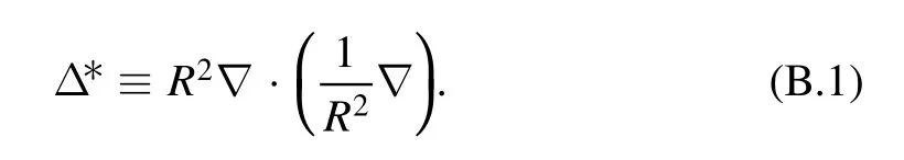
Therefore, in cylindrical coordinates (R, φ, Z) it becomes

and in flux coordinates, it becomes

whereJ and gαβ≡?α·?β are the Jacobian and the metrics of the flux coordinates respectively.

The differential operator at the magnetic axis in the local new coordinate system (u, v) defined in equation (7), can be expressed as

where (x, y) is defined in equation (6).

The Jacobian and two metrics of the flux coordinates involved in the Δ*operator can be evaluated from

They are singular at the magnetic axis and the x-point of a divertor configuration.

Appendix C.Methods for searching magnetic axis and flux surfaces

At each step during the iteration for solving the nonlinear GS equation, we get a newψkp+1(ρ,θ)k, based on which the grid positions of the flux coordinates are updated.

Gradient descent algorithm [24] is employed to find the position of magnetic axis.A schematic plot of the method for

Figure C1.A schematic plot of the method for obtaining the positions of a new magnetic flux surface.The(R 0k ,Z0k )is the position of the magnetic axis in the real space in the kth step and

(,) is the new position of the magnetic axis.The lines indicates the minor radius directions at θ=θj(black for the old one and red for new one).the dashed contours indicate the old flux surfaces at the kth step.obtaining the positions of a new magnetic flux surface is shown in figure C1.It illustrates that FEQ uses three steps to get the minor radii of new grids r(ρ, θj) at each θ=θj.

(i) The minor radii of intersections (red pluses) between the line at θk+1=θj(red line) and the old flux surfaces at kth step (black dashed contours), r|intersections, can be determined, after the position of new magnetic axis() is obtained.

(ii) The poloidal magnetic flux and the corresponding new radial coordinate at those intersections,()∣intersections, can be obtained by interpolation.

(iii) The minor radii of new grids r(ρ, θj) can then be determined using the dependence r=r(ρk+1)|intersections.

Here Piecewise Cubic Hermite Interpolating Polynomial(pchip) method is used for related interpolation.