Optimization Algorithm for Reduction the Size of Dixon Resultant Matrix: A Case Study on Mechanical Application

Shang Zhang , Seyedmehdi Karimi, Shahaboddin Shamshirband and Amir Mosavi

Abstract: In the process of eliminating variables in a symbolic polynomial system, the extraneous factors are referred to the unwanted parameters of resulting polynomial. This paper aims at reducing the number of these factors via optimizing the size of Dixon matrix. An optimal configuration of Dixon matrix would lead to the enhancement of the process of computing the resultant which uses for solving polynomial systems. To do so,an optimization algorithm along with a number of new polynomials is introduced to replace the polynomials and implement a complexity analysis. Moreover, the monomial multipliers are optimally positioned to multiply each of the polynomials. Furthermore,through practical implementation and considering standard and mechanical examples the efficiency of the method is evaluated.

Keywords: Dixon resultant matrix, symbolic polynomial system, elimination theory,optimization algorithm, computational complexity.

1 Introduction

Along with the advancement of computers, during the past few decades, the search for advanced solutions to polynomials has received renewed attention. This has been due to their importance in theoretical, as well as the practical interests including robotics [Sun(2012)], mechanics [Wang and Lian (2005)], kinematics [Zhao, Wang and Wang (2017)],computational number theory [Kovács and Paláncz (2012)], solid modeling [Tran (1998)],quantifier elimination and geometric reasoning problems [Qin, Yang, Feng et al. (2015)].Without explicitly solving for the roots, the difficulties in solving a polynomial is to identify the coefficients conditions where the system meets a set of solutions [Li (2009)].These conditions are called resultant. One possible theory, which is commonly used to find the resultant and solve a polynomial system, is elimination of the variables [Yang,Zeng and Zhang (2012)]. There are two major class of formulation for eliminating the variables of a polynomial system in matrix based methods to compute the resultants.They are called Sylvester resultant [Zhao and Fu (2010)] and Bezout-Cayley resultant[Palancz (2013); Bézout (2010)]. Both of these methods aim at eliminating n variables from n+1 polynomials via developing resultant matrices. The algorithm that adapted for this article is inspired by Dixon method which is of Bezout-Cayley type.

The Dixon method is considered as an efficient method for identifying a polynomial. This polynomial would also include the resultant of a polynomial system which in some literature is known as projection operator [Chtcherba (2003)]. Dixon method produces a dense resultant matrix which is considered as an arrangement of the non-existence of a great number of zeroes in rows and columns of the matrix. In addition, the Dixon method produces a small resultant matrix in a lower dimension. The Dixon method’s uniformity which is being implied as computing the projection operator without considering a particular set of variables is considerable properties. Besides, the method is automatic,and, therefore it eliminates the entire variables at once [Chtcherba (2003); Kapur, Saxena and Yang (1994)].

The majority of multivariate resultant methods, perform some multiplications for resultant [Faug’ere, Gianni, Lazard et al. (1992) ; Feng, Qin, Zhang et al. (2011)]. these multiplications do not deliver any insight into the solutions of the polynomial system[Saxena (1997)]. In fact, they only perform the multiplicative product of the resultant which include a number of extraneous factors. Nonetheless, these extraneous factors are not desirable resulting problems in a number of critical cases [Chtcherba (2003); Saxena(1997)]. Worth mentioning that Dixon method highly suffers from this drawback[Chtcherba and Kapur (2003); Chtcherba and Kapur (2004)].

However, in the polynomial systems, a Dixon matrix well deals with the conversion of the exponents of the polynomials [Lewis (2010)]. With this property, the Dixon method is highly capable of controlling the size of the matrix. Via utilizing this property, this research aims at optimizing the size of Dixon matrix aiming at the simplification of the solving process and gaining accuracy. In this regards, there has been similar cases reported in the literature on optimizing the Dixon resultant formulation e.g., [Chtcherba and Kapur (2004); Saxena (1997)].

This paper presents a method to finding optimally designed Dixon matrix for identifying smaller degree of the projection operator using dependency of the size of Dixon matrix to the supports of polynomials in the polynomial system, and dependency of total degree of the projection operator to the size of Dixon matrix. Having investigated these relations,some virtual polynomials have been presented to replace with original polynomials in the system to suppress the effects of supports of polynomials on each other. Applying this replacement, the support hulls of polynomials can be moved solely to find the best position to make smallest Dixon matrix. These virtual polynomials are generated by considering the widest space needed for support hulls to be moved freely without going to negative coordinate. In order to find the best position of support hulls related to each other, monomial multipliers are created to multiply to the polynomials of the system while original polynomial system is considered in the condition that the support of monomial multipliers are located in the origin. Starting from the origin and choosing all neighboring points as support of monomial multiplier for each polynomial to find smaller Dixon matrix, the steps of optimization algorithm have been created. This procedure should be done iteratively for finding a monomial multiplier set to multiply to polynomials in the system for optimizing of Dixon matrix. This will lead to less extraneous factors in the decomposed form. Further, a number of sample problems are solved using the proposed method and the results are compared with the conventional methods.

The paper is organized as follow. In Section 2, we describe the method of Dixon construction by providing the details and further evidences. In addition, an algorithm for optimizing the size of Dixon matrix has been implemented and tested in some examples,along with the complexity analysis of the optimization algorithm in this section the advantages of presented algorithm is deriving the conditions under which the support hulls of polynomials in a polynomial system do not effect on each other during the optimizing. The comparisons made with relevant optimizing heuristic of Chtcherba show the superiority of the new optimization algorithms to present the results with regards to accuracy. Finally, in the Section 3, a discussion and conclusion remarks are given

2 Methodology

In this section the optimization algorithm of the Dixon matrix and the related formulation procedure is illustrated via flowchart with some related information and theorems.

2.1 Degree of the projection operator and the size of the Dixon matrix

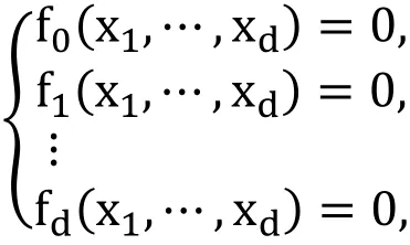
Consider a multivariate polynomial f∈ ?[c,x]. The set A ? ?d, is a finite set of exponents referred as the support of the f. Further, the polynomial system ?={f0,f1,… ,fd} , with support A= 〈A0,A1,… ,Ad〉 is named unmixed if A0=A1=…=Ad, and is called mixed otherwise. In Dixon formulation, the computed projection operator will not be able to efficiently adapt to mixed systems, and therefore, for mixed systems, the Dixon resultant formulation is almost guaranteed to produce extraneous factors. This is a direct consequence of the exact Dixon conditions theorem, presented as follow from Saxena [Saxena (1997)]:

Theorem 1.In generic d-degree cases, the determinant of the Dixon matrix, is exactly its resultant (i.e., does not have any extraneous factors).

While, generally, most of the polynomial systems are non-generic or not d-degree.

Considering simplex form of the Dixon polynomial [Chtcherba and Kapur (2004)], every entry in the Dixon matrix Θ is obviously a polynomial of the coefficients of system ?which its degree in the coefficients of any single polynomial is at most 1. Then the projection operator which is computed, is utmost of total degree |ΔA| in the coefficients of any single polynomial. Note that |ΔA| is the number of columns of Dixon matrix. A similar illustration can be presented for |ΔAˉ| (the number of rows of Dixon matrix) when the transpose of Dixon matrix be considered. Then,

is an upper bound for the degree of projection operator created using Dixon formulation in the coefficients of any single polynomial, where A and Aˉ are the supports of xs and xˉs(new variables presented in the Dixon method instruction) in the Dixon polynomial,respectively. Then minimizing the size of Dixon matrix leads to minimizing the degree of projection operator and decreasing the number of extraneous factors which exist next to the resultant.

2.2 Supports converting and its effects on Dixon matrix

The Dixon matrix size is not invariant with respect to the relative position of the support hulls (the smallest convex set of points in a support in an affine space ) of polynomials[Lewis (2010)]. In other word, the Dixon resultant matrix for a polynomial ? with the support set of A+c= 〈A0+c0,…,Ad+cd〉 is not the same as a system with support set A= 〈A0,A1,…,Ad〉, where c= 〈c0,c1,…,cd〉 and ci=(ci,1,…,ci,d) ∈ ?dfor i=0,1,… ,d. We call Ai+cithe converted support of fiand A+c= 〈A0+c0,… ,Ad+cd〉 is converted support set of polynomial system ?. However, as theorem 2 [Chtcherba(2003)], if a conversion is performed uniformly on all supports of polynomials in a system, the size of the Dixon matrix will not change.

Theorem 2. As the support for a generic polynomial system, consider A+c, where ci=cj=t=(t1,t2,…,td) for all i,j = 0,1,...,d, then

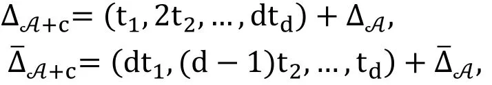
where “+” is the Minkowski sum [Chtcherba (2003)], and Δ , Δˉ are the support of Dixon polynomial for the original variables and new variables respectivly.

Consider a polynomial system ?. Assuming fi=hf′ifor some polynomials h and f′i,clearly;

where ResVis resultant of ? over verity V. In particular, if h be considered as a monomial, the points where satisfy the part ResV(f0,… ,fi-1,,h,fi+1,… ,fd) are on the axis and the degree of this resultant is not more thanwhere dmaxiis maximum total degree of fi. If we do not consider the axis, we have;

Since, we consider 1 as a variable for d+1, polynomials in d variables and the resultant computed using Dixon formulation has property (3), a polynomial in a system could be multiplied by a monomial, without changing the resultant [Chtcherba and Kapur (2004)].A direct consequence from above illustration and considering simplex form of Dixon formulation [Chtcherba and Kapur (2004)], is the sensitivity of the size of matrix to exponent of multipliers to original the polynomial system.

2.3 Optimizing method for Dixon matrix

Considering the point that, |ΔA|≠ |ΔA+t| and/or ||≠ || unless ci=cjfor all i,j=0,1,…,d from Sections 2.1, 2.2 and [Saxena (1997)], it can be said: the size of Dixon matrix depends on the position of support hulls of polynomials in relation with each other. Besides, there is an direct dependency between the area overlapped by convex hulls of polynomials and the size of Dixon matrix [Saxena (1997)].

Taking advantage of above properties, this paper intend present an optimization algorithm with conversion set c= 〈c0,c1,…,cd〉 where ci=(ci,1,…,ci,d) ∈ ?dfor i=0,1,…,d which is considered for converting the support of a polynomial system A=〈A0,A1,… ,Ad〉, to make |ΔA| and || smaller. The converted support set for polynomial system appears as A+c= 〈A0+c0,… ,Ad+cd〉. In the other words, if the polynomial system is considered in ?[c][x1…xd], the algorithm multiplies fito the monomial…to shift the polynomials support hull to find smaller Dixon matrix. The minimizing method is sequential and has initial guess for c0at the beginning.The choice of c0should be so that other cicould be chosen without getting in to negative coordinates. Then, search for c1is beginning from origin and will be continued by a trial and error method. The turn of c2is after c1when the support of multiplier for f1is fixed then, c3and so on. The process continues for finding all cis.

Not considering the effect of support hulls on each other is a disadvantage of the previous minimizing method [Chtcherba (2003)]. In fact, sometimes the effects of the support hulls on each other lead the algorithm to the wrong direction of optimization. In the other word, giving high relative distance between convex hulls of supports, the algorithm for optimizing fails and ends up with incorrect results as is noted in the end of solved examples in this section.

To suppress the effect of support hulls on each other, during of running the new algorithm presented in this paper, some polynomials should be replaced by some new polynomials, which are called virtual polynomials. The rules of selecting and using of virtual polynomials are presented in details in this section.

In the presented optimization approach, moving of support hulls of polynomials in system of coordinates is divided in four phases as;

Phase 1: Choosing c0,

Phase 2: Shifting the support hull of f0by multiplying xc0 to f0,

Phase 3: Presenting the virtual polynomials,

Phase 4: Converting of other supports.

Phase 1, 2: The space needed for executing the optimization algorithm is presented in dimension of S, where

Here, γ =(γ1,…,γd) is a d-dimensional integer vector. Considering the following polynomial system for optimization,

The choice of S is highly dependent to choice of c0that choosing bigger c0,imake the sibigger and vice versa. Whereas the complexity of the algorithm is also depending on the choice of c0, following definition for c0is presented for controlling the time complexity,however one can choose bigger elements for c0. Then c0= 〈c0,1,c0,2,…,c0,d〉 is introduced as;

The above choice for c0can be explained by the fact that it can guarantee to move other support hulls to stay in positive coordinate when they want to approach A0+c0. So the c0,ishould be chosen as above equation or bigger.

Phase 3: By searching for cpas the best monomial multiplier for fp, p=1,…,d-1 the virtual polynomials are supposed as vp+1,vp+2,… ,vdin total degrees of s,s+1,… ,s+(d-p-1) respectively, where s=. These virtual polynomials are considered without any symbolic coefficient and each one should have multifaceted vertical corner support hull. For example, in two-dimensional form ( x=(x1,x2) ), if S=(s1,s2), the following polynomial is considered as virtual polynomial to replace by f2when the algorithm intended to find optimal c1.

Having investigated the above relations, some virtual polynomials have been found to replace the original polynomials to suppress the effects of support of polynomials.Applying this replacement, the support hulls of polynomials can be moved solely to find the best position to make smallest Dixon matrix. These virtual polynomials are generated by considering the widest space needed for support hulls to be moved freely without going to negative coordinate and having effects on each other.

Phase 4: For the purpose of finding the optimal positions of support hulls related to each other, monomial multipliers are created to multiply to the polynomials of the system while original polynomial system is considered in the condition that the support of monomial multipliers are located in the origin. Starting from the origin and choosing all neighboring points as support of monomial multiplier for each polynomial to find smaller Dixon matrix, the steps of optimization algorithm have been created. This procedure should be done iteratively for finding a monomial multiplier set to multiply to polynomials in the system for optimizing of Dixon formulation.

The algorithm of the method for optimizing the size of matrix is presented by flowchart shown in following Figure.

Figure 1: Flowchart for optimizing of Dixon matrix

Here, the complexity of optimization direction for the system of polynomials ?={f0,f1,…,fd} is obtained via recognition of search area in addition to the cost of receiving better Dixon matrix in the reiterative phases. The reiterative method phases are illustrated in Fig. 1 in form of flowchart. If we consider k aswith regard to the point that for each ciwe can have maximum kd shifting, we should account Dixon matrix size in maximum kd times to arrive the best size, where we are selecting the neighboring point p (See Fig. 1, phase 4). Complexity of finding each Dixon matrix has been bounded by O(d2nd) whereWu, Tang et al. (2017);Grenet, Koiran and Portier (2013)]. Therefore, in each phase of selecting all neighboring points and considering the smallest size of the Dixon matrix, we have a complexity as O(kd3nd). For getting general answer, the optimizing direction is repeated d times as each complexity are considered for each polynomial (see the step of checking “if i=d?”in Fig. 1). Then, we have total complexity of presented algorithm as O(kd4nd).

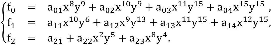
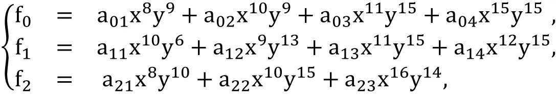
Example 1 Considering the bellow mixed polynomial system from Chtcherba[Chtcherba (2003)]:

once x,y are considered as variables and aijare parameters. The size of Dixon matrix is 99×90 which 99 and 90 regard to the number of rows and the number of columns of the matrix respectively. The polynomials support is

with support hulls

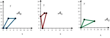
Figure 2: Support hulls of system, Ex. 1

To avoid negative exponents, we need to shift initial support A0. Using the formulation(5) we have c0=(8,9). According to the presented algorithm, we need to replace f2with virtual polynomial v2for finding a monomial multiplier for f1with support c1. Then using relation (4),

and the following polynomial system is achieved.

The size of Dixon matrix is 765×675. The above polynomials system can be considered in the case of c1=(0,0). The best monomial for multiplying to f1will be found by trial and error method as x9y6. Now when c0and c1are fixed, the f2can return to its original place and we have following system which is ready to start process for finding c2;

The size of Dixon matrix is 201×216. Using same method which is done for c1, the best monomial multiplier for f2will be found as x8y10and Dixon matrix of size 82×82.The optimal resulted polynomial system is

with optimized supports hulls which are shown in Fig. 3.

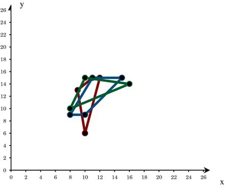
Figure 3: Support hulls of optimized system, Ex. 1

The steps of trial and error method for finding optimal c1and c2are summarized in following tables.

Table 1: Steps for finding c1 and c2 using presented method with c0=(8,9), Ex

Comparing the size of Dixon matrix after executing the algorithm and before executing in beginning of Example 1, the advantage of new presented optimizing method is evident.Optimizing the size of Dixon matrix using Chtcherba’s presented heuristic [Chtcherba(2003)] shows a big failure where the size of Dixon matrix never becomes smaller than 369×306.

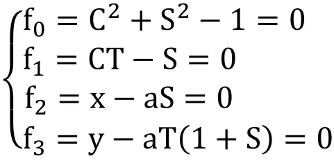
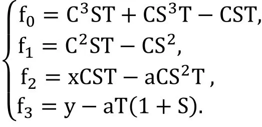
Example 2 Here the strophoid is considered. The strophoid is a curve widely studied by mathematicians in the past two century. It can be written in a parametric form described as follow.

To find an implicit equation for the strophoid using resultant, we have to restate the equations in terms of polynomials instead of trigonometric functions, as follows.

Letting S=sint,C=cost,T=tant, the trigonometric equations of the strophoid can be written as

Using the variable ordered set 〈C,S,T〉 the support sets are,

and the support hulls of polynomials is shown in Fig. 4 in system of 3-dimensions coordinate.

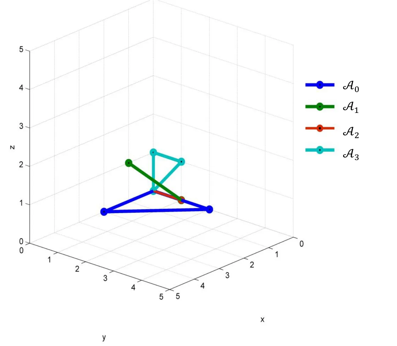
Figure 4: Support hulls of polynomials, Ex 1.2.2

For starting to search for finding best c1we introduce c0as (1,1,1) using formula (5) and replace f2,f3with virtual polynomial v2, v3respectively. Then finding the vector S is required.

Therefore, we can continue the optimizing method which is dedicated to find c1using following polynomial system.

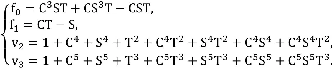
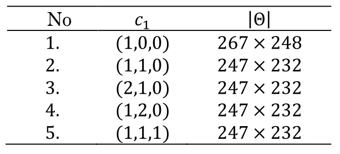
The process is summarized in the Tab. 2.

Table 2: Steps for finding c1using presented method with assumption c0=(1,1,1), Ex 2

?

The resulting polynomial system which is used for finding best c2is

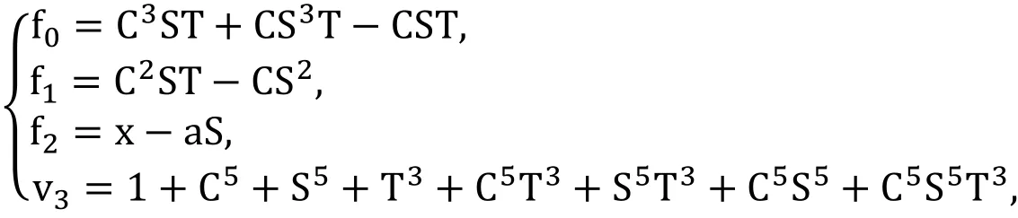
Results of algorithm with optimization are presented in the Tab. 3.

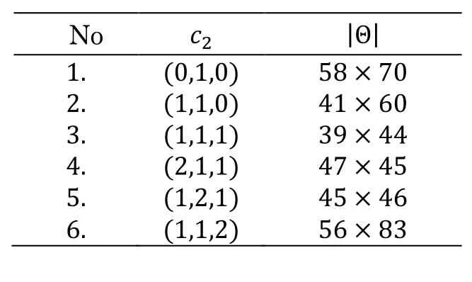
Table 3: Steps for finding c2 by new presented method, Ex 2

The process of finding best c3, which can be seen in the Tab. 4, is derived from the original polynomial system with polynomials f0,f1and f2multiplied by CST, CS and CST respectively.

The set of support hulls of optimized polynomial system is shown in Fig. 5.

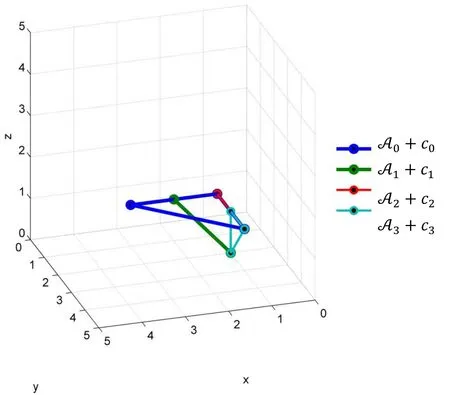
Figure 5: Support hulls of optimized polynomial system, Ex. 2

Comparing the presented result presented in Tab. 4 to the result of finding Dixon matrix[Chtcherba (2003)], which tells the Size of Dixon matrix is 6×5, we could minimize the size of Dixon matrix.

Example 3 The Stewart platform problem is a standard benchmark elimination problem of mechanical motion of certain types of robots. The quaternion formulation we present here is by Emiris [Emiris (1994)]. It contains 7 polynomials in 7 variables. Let x=[x0,x1,x2,x3] and q= [1,q1,q2,q3] be two unknown quaternions, to be determined.Let q?=[1,-q1,-q2,-q3]. Let aiand bifor i=2,…,6 be known quaternions and let αifor i=1,…,6 be six predetermined scalars. The 7 polynomials are:

Out of the 7 variables x0,x1,x2,x3,q1,q2, q3any six are to be eliminated to compute the resultant as a polynomial in the seventh. Saxena [Saxena (1997)] successfully computed the Dixon matrix of the Stewart problem by eliminating 6 variables x0,x1,x2,x3,q2,q3.The size of his Dixon matrix is 56 × 56. To optimize the Saxena’s resulted matrix, using our presented method, we should compute the c0according vector variable (x0,x1,x2,x3,q2,q3), to avoid negative coordinate. Using formula (5), the c0is (2,2,2,2,2,2). Then using formula (4), S=(6,6,6,6,6,6) which helps us to find appropriate virtual polynomials v2, …, v6as stated by details in algorithm formulation.Now we can start to fine optimal c1to present the best monomial multiplier for f1. Due to long process of finding best direction of optimizing for 6 considered variables, the process which is presented in Tab. 5 is summarized.

Table 5: Steps for finding c1 using presented method with assumption c0=(2,2,2,2,2,2),Ex 3

Then the best monomial multiplier for f1is x02x12x3q32which stand on best c1presented step number 42 in Tab. 5. Then the polynomial system can be prepared for doing the process of finding best c2by replacing v2with f2. The same trial and error method is used for finding best c2. It is found after 36 steps as (2,2,1,1,0,1) and the Dixon matrix size, at the beginning of the process, was 335×335 while at the end of optimizing process it was 286×286 . Likewise, the other supports of monomial multipliers which are known as c3, c4, c5and c6, are (2,2, 1,1,0,2), (2,1,0,2,1,1),(2,1,1,2,1,2) and (2,2,0,1,0,1) respectively, as it explained by details in [karimi (2012)].Then, in optimized form, the polynomials fi, i=0,…,6, should be multiplied by monomialsrespectively and the Dixon matrix size of optimized polynomial system is 48×48. Comparing the size of Dixon matrix according to Saxena's achieved results (as mentioned at beginning of this example), the advantage of new presented optimizing method is evident.

3 Discussion and conclusion

Though considering the simplex form of the Dixon polynomial, the maximum number of rows and columns of the Dixon matrix was presented as an upper bound of the projection operator in the coefficients of any single polynomial. In addition, since we were working on the affine space, each polynomial in a system could be multiplied by a monomial,without changing the resultant. Moreover, another useful property of the Dixon matrix construction which has been revealed was the sensitivity of the size of Dixon matrix to support hull set of the given polynomial system. Therefore, multiplying some monomials to the polynomials, which were in the original system, changed the size of the Dixon matrix yet had no effects on the resultant. It only changed the total degree of the projection operator which the resultant was a part. As long as the Dixon matrix had this property, the size of the Dixon matrix was able to be optimized by properly selecting the multipliers for polynomials in the system. Using this property, this paper sought to optimize the size of the Dixon matrix for the purpose of enhancing the efficiency of the solving process and identifying better results. Via considering the properties of Dixon formulation, it was concluded that, the size of Dixon matrix depends on the position of support hulls of the polynomials in relation with each other.

Furthermore, in order to suppress the effects of supports hulls of polynomials on each other,some virtual polynomials had been introduced to replace the original polynomials in the system. Applying this replacement, the support hulls of polynomials could be moved solely to find the best position to make smallest Dixon matrix. These virtual polynomials were generated by considering the biggest space needed for support hulls to be moved freely without going to negative coordinate. For the purpose to identify the optimal position of support hulls related to each other, monomial multipliers were created to multiply to the polynomials of the system while original polynomial system was considered on provided that the support of monomial multipliers were located in the origin.

The complexity analyses was performed for the corresponding algorithm namely the minimization method of the resultant matrix for the system of polynomials ?={f0,f1,…,fd} considered by recognition of search area along with the time cost of receiving better Dixon matrix in every single phase.

For verifying the results by implementing the presented algorithm for optimizing the Dixon matrix for general polynomial systems, the algorithm was implemented and its applicability was demonstrated in example 1 (2 dimensions), example 2 (3 dimensions)and example 3 (6 dimensions). The results of the method for minimizing the size of Dixon resultant matrix were presented in tables that reveal the advantages and the practicality of the new method. Even if we had the optimal position of support hulls at the outset, the algorithm worked properly.