Survival analysis for observational and clustered data: an application for assessing individual and environmental risk factors for suicide

Kerry Louise KNOX, Alina BAJORSKA, Changyong FENG, Wan TANG, Pan WU, Xin Ming TU,*

·Biostatistics in psychiatry （15）·

Survival analysis for observational and clustered data: an application for assessing individual and environmental risk factors for suicide

Kerry Louise KNOX1,2, Alina BAJORSKA2, Changyong FENG3, Wan TANG3, Pan WU3, Xin Ming TU1,2,3*

1. Introduction

Survival analysis concerns the time from a well-defined origin to some event of interest, such as the time from surgery to death of a cancer patient, the time from wedding to divorce, and the time between the first and second suicide attempts. Although originated in research on the active lifetime of light bulbs and other electric devices, modern applications of survival analysis include many non-survival events. Thus, survival analysis may be more appropriately called the time-to-event analysis.

Like all other statistical methods, survival analysis deals with random events such as death, divorce and suicide. Thus, the time to the event of interest is a nonnegative random variable, and usually right skewed because most events tend to occur in close proximity to each other after a period of time. In survival analysis we are primarily interested in the distribution of survival time and the influence on such a distribution of some explanatory variables such as age and gender. In some applications, data may also be clustered, or correlated,because of certain common features such as genetic traits or shared environmental factors. Clustered survival time data also arise from analyses involving multiple occurrences of an event from the same individual, such as repeated suicide attempts.

Unlike their applications in randomized controlled trials, there are more issues to consider when applying survival analysis to observational data. To illustrate the principles involved, this article uses data from a study of the United States Air Force (USAF) active duty personnel during fiscal years 2004-2009, focusing on suicide in this population and on their utilization of medical services.We discuss how to assess the effect of demographic characteristics (e.g., gender), time-dependent factors(e.g., job characteristics), and changes of mental health conditions (e.g., depression and anxiety) on the risk of suicide. We also discuss how to analyze the impact of shared environmental factors such as organizational culture on the risk of suicide by accounting for data clustering due to nested data structures.

2. Data sources and study population

2.1 Data sources

Our research population comprises approximately half a million USAF active duty members who were in service within a 6-year period between October 2003 and September 2009. Information about the population has been extracted from several data sources maintained by military centers. The personnel database, a part of the Military Personnel Data Systems managed by the USAF Personnel Center and updated monthly, was the source of individuals’ socio-demographic and jobrelated information for our analysis. The suicide event database maintained by the Suicide Event Surveillance System was used to identify suicide victims and time of suicide. Information on utilization of medical services was taken from four databases from the Military Health System’s Military Data Repository, which contained two outpatient medical care data sets and two inpatient medical care data sets:

· Standard Ambulatory Data Record (SADR)for all ambulatory care provided in military facilities;

· Health Care Service Record, Non-Institutional(HCSR-NI) for ambulatory care provided to USAF personnel in civilian facilities;

· Standard Inpatient Data Record (SIDR) for inpatient care provided in military facilities;

· Health Care Service Record, Institutional(HCSR-I) for inpatient care provided to USAF personnel in civilian facilities.

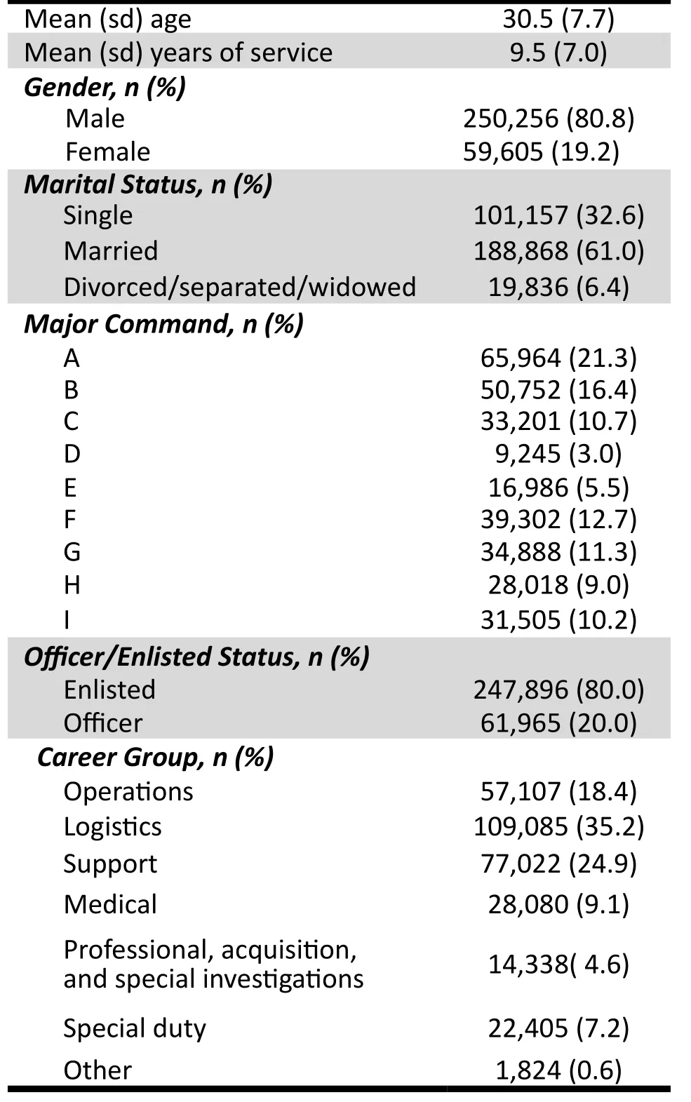
Table 1. Characteristics of the cohort（309,861 servicemen） as of October 2006

We extracted service utilization information from the above files for the period October 2000 through September 2009, except for the outpatient HCSR,which was based on the period October 2001 through September 2009. In all data sources, individuals’ real identifiers, such as their social security number, were replaced with artificial pseudo identifiers created by the agency that provided the data which identified each individual’s records within and across the files.This study received approvals from Institutional Review Boards at the USAF, Wilford Hall and the University of Rochester.

2.2 Characteristics of the study population

The characteristics of USAF active duty personnel as of October 2006, the midpoint of the study period, are shown in Table 1. Eighty-one percent were men, their mean (sd) age was 30.5 (7.7) and their mean duration of service was 9.5 (7.0) years. Most were married (61%),and a small proportion (6%) were divorced or widowed.Twenty percent were officers. Career groups represented different types of occupations. The personnel were distributed across 84 USAF bases organized into 9 Major Commands (one of the major command groups includes all personnel located outside of USAF bases).

Average suicide rates for the entire study population and for demographic subgroups of the population are shown in Table 2. The rate was calculated by dividing the number of suicides that occurred during the study period by the total exposure time, and then multiplying the result by 100,000. For example, first dividing 227 suicides by 1,961,247 person-years and then multiplying the result by 100,000, we obtained the average rate of 11.6 suicides per 100 000 person-years for the study population. To compare relative rates between women and men, we obtained a rate ratio of 0.248, unadjusted for other factors, indicating that the rate of suicide for women was about one fourth of that for men. Similarly,we calculated the rate ratios for different age groups and for groups defined by different marital status. For age, we partitioned the study population based on the quartiles of the age distribution and used the first quartile as the referent for comparison.

Using survival analysis methods (discussed in Section 3), we computed the 95% confidence interval for each rate ratio shown in Table 2. Age appeared significantly protective of suicide, that is, the rate was lower for older people than for younger people, when uncontrolled for other factors. Married individuals had a significantly lower suicide rate compared to their single and divorced or widowed counterparts; the rate in the divorced or widowed group was higher than among those who were single. However, these results may be confounded by age, since single people were generally younger than married ones, so the married status may simply be a correlate of age.

3. Survival analysis methods for assessing risks of suicide

3.1 Rate of suicide and proportional hazards model

The rate of occurrence of a disease in epidemiologic research is often calculated as the ratio of the number of cases to total exposure time, as shown in Table 2. This measure integrates the number of suicide cases with total observation years from all subjects. This is a more sensible index than the percent, or proportion, of people who committed suicide, since it takes into account the length of observation time. However, the use of length of observation time as the denominator makes it more complicated (than in the case where number of individuals is the denominator) to assess the variability of the rate and the standard errors and confidence intervals for the rate. In this situation, the usual statistical methods for proportions cannot be used to provide confidence intervals. Further, the rates shown in Table 2 reflect the average risk of suicide over a period of 6years, rates that could have changed significantly during this period. Even within a subgroup, the likelihood of committing suicide could have varied substantially across the subjects over time as well. To address the statistical issue and to estimate ‘instantaneous’ risk at any point in time, survival analysis methods are needed to model temporal patterns and between-subject variability in suicide risk.

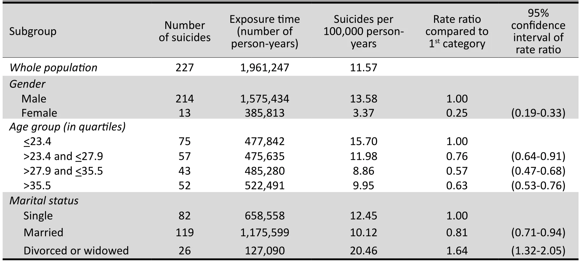
Table 2. Rate of suicide for the study population and for subgroups in the study population

To reflect the changing risk of suicide over time, we fix the time origin, such as the time of entry to USAF, and use T to denote the lapse of time from the time origin to suicide. We then compute an average rate of suicide per person-year over a small interval, say (t,t+Δt), around a time point T=t, by dividing the number of suicides within the interval by the sum of observation times across all individuals still under observation by time t+Δt, that is,

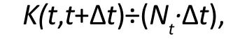
where K(t,t+Δt) is the number of suicides that occur within the interval and N,is the number of people still at risk (alive) at the time t. As the interval shrinks to the point t, we obtain, by using a mathematical argument, an instantaneous rate of suicide per person-year at time t:

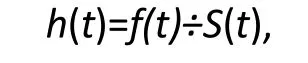
where f(t) is the probability density function, S(t)=1-F(t) is the survivor function and F(t) is the distribution function of T.

The value h(t) is also known as the hazard function,which within our context describes an individual’s risk of suicide at time t. The hazard function is completely determined by the distribution function F(t)of T and vice versa. In most applications including our context, we model the hazard function, since it is a more meaningful and interpretable quantity.

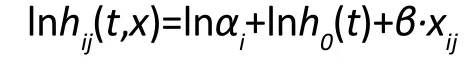
The commonly used approach for modeling temporal trend and between-subject variability is the proportional hazards model. If x denotes an explanatory variable such as gender or age at entry to USAF, the hazard function under this popular model is given by:

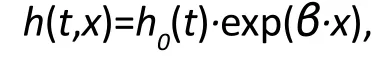
or equivalently when expressed on the log scale,

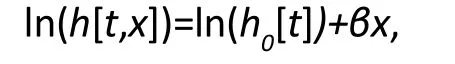
where h0(t) is the baseline hazard function, that is, the hazard in the absence of x. The hazard ratio exp(?)represents the effect of x on the hazard function per unit increase in x.

Note that the effect of x on the hazard in this model is multiplicative and constant across time. For example,if x is a binary indicator with x=1 (0) representing female(male), the baseline hazard h0(t) represents the hazard of suicide for males over the duration of service, while the regression part, exp(?), is the hazard ratio (or relative hazard or risk score) for females compared to males.As another example, if x is deviation from average age at entry, the baseline hazard is the risk of suicide for an individual with this mean age, while h(t,x) is the hazard for a person x years older (x＞0) or younger (x＜0) at entry to USAF.

The proportional hazards model is easily extended to include multiple explanatory variables. If xkdenotes a kthvariable for an individual (1≤k≤K), the hazard of suicide for the person is given by:

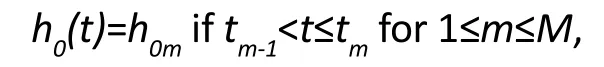
The baseline hazard h0(t) can be parametrically modeled or left unspecified. An example of the parametric approach is a piecewise constant baseline hazard over time. Under this model, the observation period is divided into segments and within each time interval the hazard is constant. If we partition the study period into M intervals, t0＜t1K≤tMand denote by h0mthe constant baseline hazard in the mthinterval, the piecewise constant baseline hazard has the form:

In many applications, the baseline hazard is left unspecified, giving rise to the semi-parametric Cox proportional hazards model in the sense that h(t,x)has both a non-parametric baseline hazard h0(t) and aparametric component for the effects of explanatory variables. In the Cox regression model,the unspecified baseline hazard h0(t) is estimated empirically. If the interval is very small in the piecewise constant baseline hazard model, there will be little difference between the parametric and semi-parametric Cox proportional hazards models. The baseline hazard function from the latter model is approximated by the piecewise constant function of the former, with improved precision when smaller intervals are used. Thus, it is better to employ the piecewise constant baseline hazard model when significant variability of baseline hazard can be well described through a sparse partition of the study period, such as years or quarters in our context.

3.2 Inference of model parameters

In order to estimate effects of explanatory variables xkin the proportional hazards model, we need observed values of the failure time T(x1,K,xk) for all subjects in the sample. For individuals who commit suicide, T(x1,K,xk) is the time when the event occurred. But for most people who do not die of suicide, they are right censored at time c, where c is the last time the subject is observed,either at the end of the study period or at the time of discharge from the USAF. For such censored subjects, we only know that their failure times are greater than c, that is, T(x1,K,xk)＞c.

A standard approach for inference about parameters is the maximum likelihood. The maximum likelihood estimate is the value of the parameters that maximizes the likelihood function, which is the probability of observing the failure times T(x1,K,xk) in a study sample.For those who die by suicide, T(x1,K,xk) is the time of suicide, while for those who are censored, T(x1,K,xk) is set to c. An event indicator d is used to distinguish suicide,d=1, from censored events, d=0.

For the proportional hazards model, the set of parameters, ?k, is of primary interest. As noted earlier,we may either specify a particular form for the baseline hazard h0(t) such as the piecewise constant model or leave it unspecified as in the Cox proportional hazards model. Regardless of how h0(t) is modeled, we obtain estimates of both ?kand h0(t); the only difference is that if h0(t) is specified, the modeled baseline hazard function is estimated, and otherwise, an empirical version of the baseline hazards is provided.

3.3 Time-dependent explanatory variables

When modeling data from studies with long durations,such as in the study of the natural history of a disease or a condition such as suicide, some important characteristics of the study sample may change significantly during the course of the study and it is important to take such changes into consideration. For example, our study was 6 years long during which time an individual might get promoted (from the enlisted to the officer status) or relocated to a different base or Major Command group.To account for such time-varying, or time-dependent,explanatory variables, we modify the proportional hazards model as follows:

where xk(t) describes each person’s characteristics at time t. For example, if an individual joins the USAF as an enlisted serviceman and three years later gets promoted to officer status, we use a time-varying indicator x(t)to denote the change of status, with x(t)=0 for t≤3 before and x(t)=1 for t＞3 after the change. This person’s hazard will change from h0(t) during the first 3 years to h0(t)·exp(?) after the promotion.

Sometimes, a variable can be either coded as a time-invariant or time-varying variable, depending on the purpose of the analysis. For example, in the officer versus enlisted status case, if we want to know whether the original status at the entry affects a person’s hazard of suicide, the enlisted versus officer status at entry to service will be coded as a time-invariant variable. The effect of this variable indicates differential risks of suicide between enlisted and officer status at entry to service.

3.4 Choice of time origin and its implications

In most clinical trial studies, the origin of the failure time T(x1,K,xk) is typically set at the start of the study or at entry to the study if patients enter the study at different times. However, when modeling the natural history of a disease using observational data such as suicide,there are more options for selecting this time origin.Depending on the choice of starting time, the baseline hazard describes changes for different reasons and, as such, must be interpreted accordingly.

In the context of the study of suicide, when the time origin is entry to USAF, the baseline hazard h0(t)describes how the rate of suicide changes during service.Thus, the regression part of the model cannot include the duration of service variable, but can contain variables to model temporal fluctuations of risk of suicide specific to calendar-times such as seasonality.Alternatively, if the time origin is set at the beginning of the study (October 2003) the baseline hazard reflects temporal fluctuations such as seasonality and thus the regression part can include variables on duration of service, but not on temporal variability during the study period.

The choice of the time origin also has significant implications for the interpretation of variables in the regression part of the proportional hazards models. For example, if October 2003 is set as the time origin, then an individual’s age at this time origin (z1), is the person’s age at entry to service (x1) plus his or her duration of service at the time of origin (x2); thus, z1=x1+x2. The two age variables, z1and x1, will have implications for model estimates. To illustrate, let us suppose that we model risk of suicide using only age and duration of service as the explanatory variables. Then, the hazard for the age variable z1defined as October 2003 is given by:t,z1,x2)=h0(t)·exp(Y1·z1+Y2·x2)=h0(t)·exp(Y1·x1+[Y1+Y2]·x2),

while the hazard for the age variable x1defined at entry to service is:

By comparing the parameters, we see that Y1=?1and Y1+Y2=?2. Thus, although the change of definition does not affect the parameter estimate associated with age, it does alter the interpretation of the variable of duration of service x2. In this particular example, when used with age at entry to service, the hazard ratio (HR) of duration of service exp(?2) is equal to exp(Y1+Y2), the HR of age at October 2003 exp(Y1) times the HR of duration of service exp(Y2).

3.5 Censoring and competing risks

In order to make correct inference about a population in the presence of censoring, the uncensored observations must be representative of the whole study population. In other words, the censoring mechanism cannot operate selectively and censor subjects with unusually high (or low) risk for the event of interest. Under independent censoring assumption, censoring is independent of the failure time T; that is, the failure time has the same distribution for the events observed as for the censored observations (had they been observed beyond the censoring time).

In our suicide study, in addition to censoring due to the limited study period, suicides might also have been censored by competing risks such as discharge from service, change of status from active duty to reserve or guard duty, and death from other causes. Some of these competing risks may cause dependent censoring,in which case the censored cases may have a higher (or lower) risk of the event. For example, discharge from the USAF may be a dependent censoring mechanism if individuals with mental health problems are more likely to be discharged than those without mental health problems. To assess such potential bias, we may perform sensitivity analysis by including suicides that occurred shortly after separation from active duty (e.g., up to 6 months after discharge). To find suicide cases among individuals discharged from the USAF, one may use the US National Death Index, the nationwide central index of death record information.

Some suicides might also have been misclassified as accidental deaths, since the victim and possibly his or her commanders might be interested in disguising suicide deaths. Therefore additional analyses of accidental or violent deaths may also be useful in assessing potential bias due to dependent censoring. Since suicide is a rare event, the analyses of results may also be sensitive to errors in reporting.

3.6 Accounting for data clustering

Like other statistical models, survival analysis also relies on stochastic independence across subjects for valid inference. If observations within some group are correlated because of certain common features such as genetic traits or shared environmental factors, estimates of model parameters obtained from maximum likelihood may still be valid, but estimates of standard errors and associated confidence intervals are generally not. In our study, the data are clustered by the USAF bases as well as the Major Commands, because of shared environmental and social factors such as specific job demands,geographic locations, and the heightened awareness and detection of early signs of suicide by some bases (but not by all bases).

One way to correct the bias introduced by such clustering is to use sandwich, or empirical, variance estimates. This robust variance estimate addresses bias‘post-hoc’ in the sense that the effect of data clustering is dealt with at the inference stage. An alternative is to model the correlation directly. The shared frailty model follows the latter path by explicitly modeling data clustering through random effects, or latent variables.

Under the shared frailty model, the correlation within a cluster is modeled by a cluster-specific effect, or shared frailty, αi, in the hazard function:

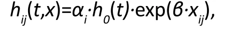
where i ranges over the different clusters and j iterates over the subjects within in the ithcluster. Under this approach, the random effects αiare assumed independent, following a gamma distribution with a mean equal to 1. When αi＞1 (αi＜1), it implies that individuals in the ithcluster have higher (lower) hazard compared to a cluster with the average frailty αi=1. The variance of αimeasures the variability across the clusters,with a larger value indicating higher between-cluster variability (or within-cluster correlation). We might write the same model on the log hazard scale:

In this form, the shared frailty model resembles a standard random effects regression model with groupspecific random intercept, which is widely used in other contexts of clustered data such as longitudinal data analysis.

When analyzing clustered data, it is important to have a large number of clusters, especially when the between-cluster variability is high, since accuracy of estimates is largely determined by the number of clusters. Within our context, there are two levels of data clustering, bases and Major Commands, with bases nested within Major Commands. Because there are only 9 Major Commands, but 84 bases, we addressed the base-clustering effect using the above cluster-specific methods (sandwich variance estimate and shared frailty model), while accounting for variability between Major Commands using fixed-effects, that is, by treating Major Commands as 9 subgroups.

4. Application of survival models to examine risks of suicide

The data for our study cohort was based on the personnel files extracted from the Military Personnel database. We utilized multiple monthly records per individual in our analysis. The individual’s first monthly record within the study period (October 2003 or entry month if the individual joined the USAF after October 2003) included full study-relevant information about the person. Personnel records for the subsequent months included only new information when changes occurred in the personnel data. The last record for the individual marked the end of the study period (September 2009)or the end of individual’s personnel data if the individual was separated from active duty before the end of study period.

The data included individuals’ socio-demographic and job-related characteristics such as gender, age,marital status, officer or enlisted status, duration of service in the USAF, career group, location (bases), and Major Command (groups of USAF bases). The time was measured in years elapsed from the time origin selected such as the beginning of the study or entry to USAF. If using entry to USAF (October 2003) as the time origin,the time 0 refers to entry to service (October 2003).

The analytical file was created in the counting process input style, a common file format for many popular statistical packages such as SAS and STATA. The observation period for each person was divided into a set of periods reflecting the changes of time-varying variables so that all time-varying and time-invariant variables became constant within each period. Thus,each individual had multiple lines of data, with each line representing a different period, beginning with the first and ending with the last period. For example, if a person joined the USAF as enlisted and three years later got promoted to officer status, this person would have at least two lines of data. In the first line, the time-varying status indicator, x(t)=0, indicating the referent’s enlisted status before the change, while in the second line, x(t)=1,denoting the new officer status beginning in year 4. If there are multiple time-varying variables, the number of lines is defined by the different combinations of the variables so that each line represents a period within which all the time-varying variables assume a constant value.

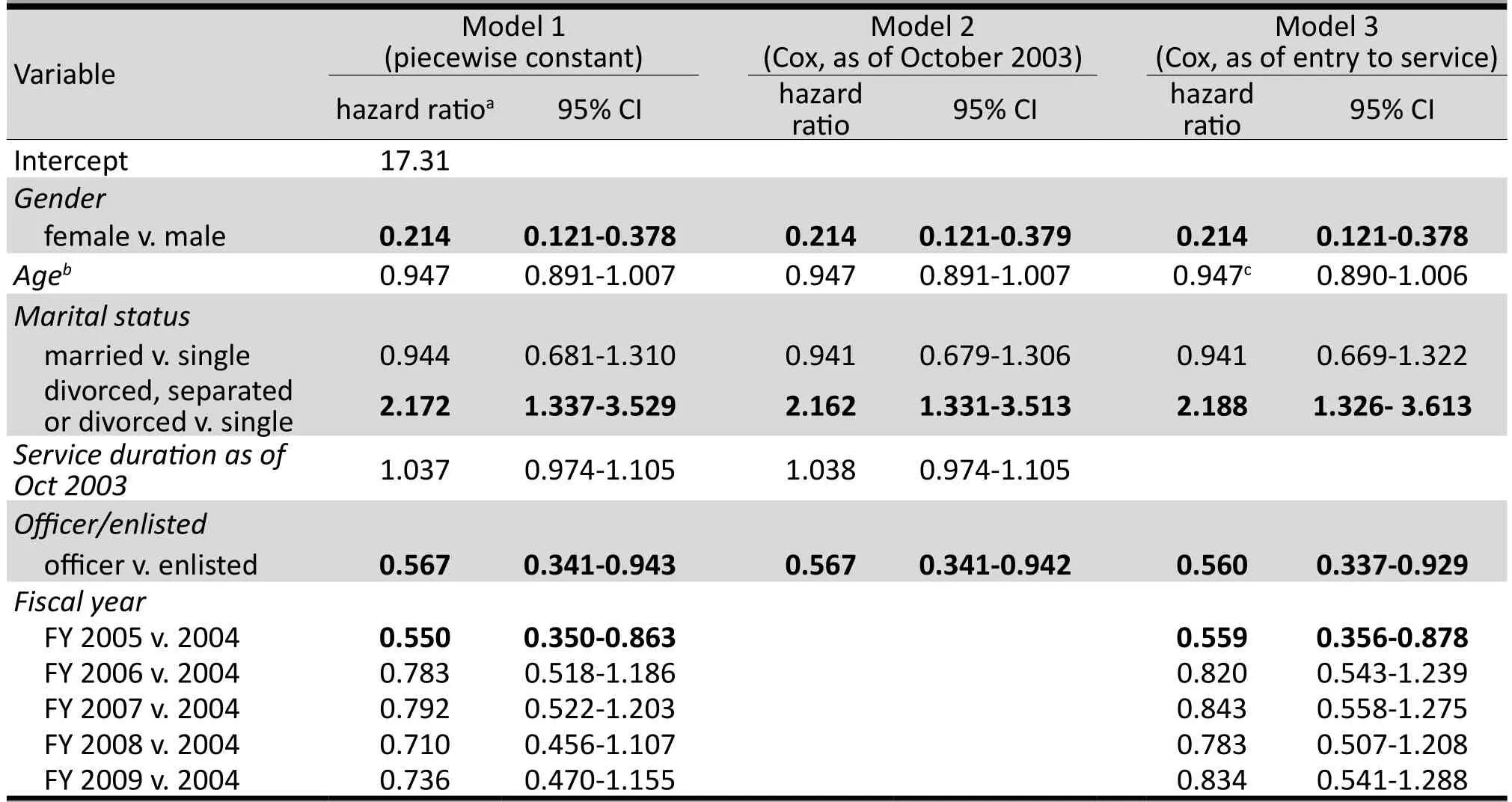
Table 3. Comparison of hazard ratios of piecewise constant baseline hazard （Model 1） and Cox models （Models 2 and 3） with time origin set at October 2003 （Models 1 and 2） and entry to service （Model 3）

4.1 Demographic variables

We first focused on demographic variables. We used two different time origins to illustrate how interpretations of model estimates would change with the two choices of time origin discussed above. We considered three survival models. The first (Model 1) was a piecewise constant baseline hazard model, with the beginning of the study period (October 2003) as the time origin and fiscal years entered as discrete-time indicators to control for temporal changes in the hazard. The other two models were Cox proportional hazards models with two different time origins ? the beginning of the study period(Model 2) and the time of entry to USAF (Model 3).

Although Models 1 and 2 used the same time origin,the regression part of Model 2 could not contain the indicators of fiscal years, since such temporal changes were accounted for by the (unspecified) baseline hazard.For Model 3, the service duration variable could not be included in the regression component because the(unspecified) baseline hazard of the Cox model accounted for the changes of service duration (from the time of entry into the USAF), but the regression did include the indicators of fiscal years which modeled temporal changes in hazard of suicide during the study period, October 2003-September 2009.

Model 1 is identical to Model 2, except that Model 1 explicitly models the baseline hazard using a constant value within each 1-year interval, rather than leaving it completely unrestricted, as is done in Model 2. The estimated baseline hazard is shown in Table 4, along with the estimates for the demographic variables. The intercept 17.31 per 100,000 person-years represented the baseline hazard of suicide for the 2004 fiscal year for a single, 26-year old enlisted man at the entry to the service. The hazards for the remaining fiscal years can be calculated by multiplying the 2004 rate by the estimated hazard ratios. Since the hazard ratios were smaller than one, the remaining fiscal years all had lower hazards than the referent fiscal year 2004. However, only the 2005 rate was significantly lower.

All three models yielded quite similar results.Although the age variable was defined differently in Models 2 and 3, its interpretation remains the same;it represents the effect on the hazard function per unit(year) increase in age.

4.2 Age and duration of service

Age was set at the time origin (October 2003) for Models 1 and 2 and at entry to service for Model 3. In Section 3.4,we discussed how different definitions of age would alter interpretations of estimates for other variables. We now illustrate such considerations with the real study data.

To this end, we ref i t Model 2 above by re-setting age to the age at the time of entry to service. The estimated age effect of this new model (Model 5) is shown in Table 4, compared to the original age effect of Model 2, which is labeled ‘Model 4’ in the table. The age variable in both models is interpreted the same way as the effect of being 1 year older at any time t on the hazard of suicide. The effect and interpretation of service duration, however,is different between the two models. In Model 4, the effect represents an increased risk of suicide (HR=1.038,albeit not significant) for each additional year of service for two people with the same age. In Model 5, such an interpretation does not work, since two people who joined the USAF at the same age also had the same years of service. As discussed in Section 3.4, the HR in Model 5 is the product of the service duration HR and age HR from Model 4. So this “aging while in service” phenomenon is the effect of two polarizing factors, with ‘a(chǎn)ge’ reducing and‘service’ increasing the risk of suicide.

4.3 Mental disorder diagnoses

We next examined whether mental disorders were predictive of suicide. We considered three mental disorders: any mood disorder (mainly depression), any anxiety disorder, or any substance use disorder (mainly alcohol abuse or dependency). We used codes from the ninth edition of the International Classification of Diseases(ICD-9) to identify treatments for the three broad mental disorders:

· Any mood disorder identified by codes for depression or bipolar disorder;

· Any anxiety disorder identified by codes for anxiety or Post Traumatic Stress Disorder(PTSD);

· Any substance disorder identified by codes for alcohol or other substance abuse or dependency.

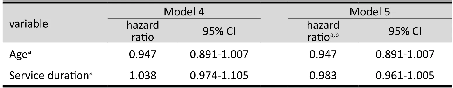
Table 4. Comparison of estimates of service duration between two definitions of age with one defined as October 2003 （Model 4）and the other at entry to service （Model 5）

Table 5A. Cox proportional hazard model for suicide with mental disorders diagnoses as risk factors, adjusted for socio-demographic and job related characteristics （Estimated effects of socio-demographic and job related characteristics)

We refer to the three categories as mood, anxiety and substance disorders. We wanted to know not only if any of these conditions would predict suicide, but also the timing of the effect, that is, if suicide was more likely to occur within the first year of the episode compared to the subsequent period. In identifying episodes of mental disorders, we used all types of medical care utilization:outpatient and inpatient encounters in either military or civilian settings.

The concept of the episode originated from the idea of an individual’s first treatment encounter that included a specif i ed diagnosis. Due to limitations of the dataset, however, it was not possible to establish the time when the very first encounter occurred. Instead,we determined the first encounter based on a two-year window determined by the availability of the treatment history across the inpatient/outpatient and civilian/military databases. After two years of no encounter with the treatment services, the clock was reset to 0 and a new encounter was established as the beginning of a new episode. Thus, the beginning of a new episode of the disorder was defined as a treatment encounter preceded by at least a two-year period of no treatment for this disorder. Likewise, the end of the spell was defined as two years after the last treatment of the episode.

The mood and anxiety disorder variables were categorical, each with the value 0 if the individual was not in an ongoing episode, 1 if the individual was in the first year of the episode, and 2 if the individual was in the second or subsequent years of the episode. Due to fewer events, substance disorder was dichotomized with value 0 if not in an ongoing episode and 1 if the in first or subsequent years of the episode. The three mental disorder variables were all time-varying variables toreflect the changing status of the disorders over time.

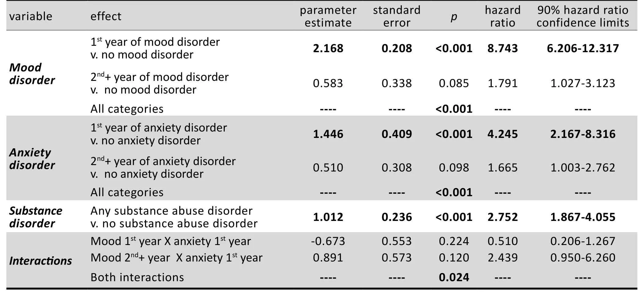
Table 5B. Cox proportional hazard model for suicide with mental disorders diagnoses as risk factors, adjusted for socio-demographic and job related characteristics （Estimated effects of mental disorders.）

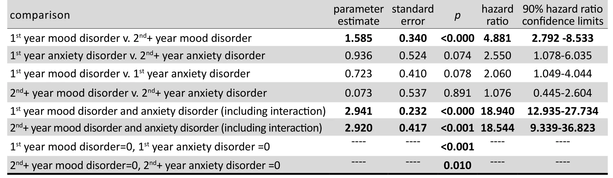
Table 5C. Cox proportional hazard model for suicide with mental disorders diagnoses as risk factors, adjusted for socio-demographic and job related characteristics （Comparison of effects of duration of an episode within the same disorder and between the different disorders）

To evaluate how the hazard of suicide depends on the mental disorders while controlling for sociodemographic and job characteristics, we performed the Cox proportional hazards model with October 2003 as the time origin. We created four age groups based on the quartiles of age distribution at entry to service and used the first quartile as the referent comparison group. The same approach was used for creating the groups of service duration. We also controlled for the effect of Major Commands through fixed effects, while accounting for intra-base correlations through the sandwich variance estimate.

The estimated hazard ratios for the demographic variables are shown in Table 5A, those for mental disorders are shown in Table 5B, and differential effects of duration of an episode (e.g., first year vs. second year of mood) within the same disorder as well as between the disorders is shown in Table 5C.

As shown in Table 5A, age, gender, marital status,duration of service, officer status, and major command were all significantly associated with risk of suicide.Women were at lower risk (HR=0.16, p＜0.001), and divorced or widowed service members had twice the hazard of suicide compared to single or married individuals. The effect of age was protective; for example, being in the third quartile of age (28-35.5 years) decreased the risk of suicide by approximately 60% (HR=0.417, p=0.002) compared to the youngest(referent) group. When controlling for age and other factors, longer service duration increased the risk of suicide: individuals with more than 14 years of service had about twice the risk of suicide compared to the group with at most 6.8 years of service. Officer status was also protective.

Table 5B shows that episodes of mood, anxiety or substance disorder increased the risk of suicide. The hazard of suicide was almost 8.7 (p＜0.001) times higher for an individual in the first year of a mood episode(without concurrent anxiety) than someone without an ongoing episode of a mood disorder, all other things being equal. The hazard ratio (HR) for anxiety in the first year (without mood) was 4.2 (p＜0.001). There are two interaction terms in the bottom three rows of Table 5B. The estimated coefficient for the interaction term of Mood 1styear and Anxiety 1styear is negative(-0.673), implying that the risk of suicide death for a subject with both a 1styear mood disorder and a 1styear anxiety disorder is less than the combined risk of the two disorders (that is, overall risk=2.168+1.446-0.673=2.941;shown in Table 5C); but this overall risk of 2.941 is greater than the risk of someone with either a 1styear mood disorder (risk=2.168) or a 1styear anxiety disorder(risk=1.446), all other things being equal. On the other hand, the interaction term for the Mood 2nd+ year and Anxiety 1styear is positive (0.891), indicating that the concurrent presence of a 2nd+ year mood disorder and a 1styear anxiety disorder magnifies the risk of suicide to a value greater than the combined risk of the two disorders(that is, overall risk=0.583+1.446+0.891=2.920; shown in Table 5C), all other things being equal.

Table 5C shows that for both mood and anxiety disorders the first year of the episode was associated with a higher risk of suicide than subsequent years: HRs were 4.9 (8.7/1.8) (p＜0.001) for mood and 2.6 (4.2/1.7)(p=0.07) for anxiety. The first year of a mood episode was more predictive of suicide than the first year of an anxiety episode; HR=2.1 (p=0.08), but the difference in hazard for suicide between mood episodes and anxiety episodes disappeared after the first year of the episodes. The final two rows of Table 5C provide the statistical significance of two composite null hypotheses. The second-to-last row indicates the probability that individuals with either a 1styear mood disorder or a 1styear anxiety disorder or both type of disorders are at the same risk of suicide (i.e.,both have a coefficient of zero) as all other individuals.The final row indicates the probability that individuals with either a 2nd+ year mood disorder or a 2nd+ year anxiety disorder or both types of disorders are at the same risk of suicide as all other individuals. The p-values for both of these composite null hypotheses are ＜0.05,which indicates that these hypotheses are rejected; that is, these disorders are significantly associated with the risk of suicide.

Note that when factors are closely linked and change together (e.g., longer service is associated with older age), they should be included together in the model and interpreted with respect to each other. For example,when age was not included in the model, the effect of longer service became protective of suicide; but when both age and length of service are included in the model,age is a protective factor and length of service is a risk factor for suicide. Thus, when factors are closely linked,exclusion of one of the factors can result in misleading interpretation of the remaining factors.

4.4 Variation across bases and major commands

The effect coding was used to create dummy indicators of the different Major Commands in the analysis. Under this coding scheme, the baseline hazard represents the mean, or average, effect over all nine Major Commands,while each dummy indicator of Major Command shows the difference between the corresponding Major Command and the mean effect of all Major commands.

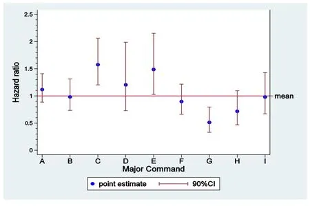
Figure 1. Hazard ratio of suicide by each Major Commandcompared to mean hazard of all Major Commands

There was significant variability in the hazard of suicide across the 9 Major Commands (p=0.026), as shown in Table 5A. Figure 1 also depicts the hazard ratios of the 9 Major Commands compared to the baseline hazard, along with a 90% CI of the baseline hazard. We can see that hazards of suicide were significantly higher at Major Commands C and E, but were significantly lower at Major Command G.

Since the sandwich variance estimate used in the above analysis addresses data clustering at the base level ‘implicitly’ through estimation, we could not obtain estimates of variability across the bases. To get some ideas about the latter variability, we ref i t the data with the shared frailty model. We obtained quite similar estimates for all the variables reported in Tables 5A,5B and 5C. However, the shared frailty model yielded additional information about the variability of suicide at the base level. The estimated variance of the Gamma random effect αiwas 0.023, which was significantly different from 0 (p＜0.001). Thus, there was significant variability in suicide across the 84 USAF bases.

5. Comparison of methods and software packages

We discussed a range of models for survival data and their applications to modeling suicide using observational data. With piecewise constant baseline hazard and Cox models, we can model effects of multiple risk or protective variables on suicide and even account for correlated outcomes using robust variance estimates or shared frailty. One advantage of the piecewise constant baseline hazard model over the Cox model is shorter computing times. Another is a direct control of the baseline hazard, providing the ability to model temporal trends specific to a study such as fiscal years in our application. However, as it requires dividing the study period into smaller time intervals, the piecewise constant baseline hazard model demands additional programming efforts which, depending on how refined the time intervals are, may result in very large files,potentially exceeding limited memory capacity.

We used SAS and STATA packages to prepare data and perform model fitting for all the examples. The two packages are similar in many respects, but there are also some differences. In our application, we found that when fitting the Cox model, it took longer for SAS (version 9.2)than STATA (version 8) to obtain model estimates. In addition, STATA has convenient built-in commands for splitting records and performing other manipulations necessary to create appropriate file structures for fitting survival models. A shared frailty option is also available in Stata when fitting the Cox as well as fully parametric models such as the piecewise constant baseline hazard model. The sandwich variance estimate is available in either software package. One advantage of SAS is that the results are presented in nice-looking tables.

6. Discussion

We have discussed how to assess effects of individual and environmental factors on the rate of a disease using survival analysis methods. We started with simple calculations of rates, but finished the discussion with quite complex survival analysis models. By using data from a real observational study on risk of suicide, we have introduced not only the basic elements of the modeling theory, but also important considerations such as selection of time of origin and data clustering when modeling the natural history of a disease such as suicide.With respect to the USAF study population in our analysis, we found that mental disorders such as mood disorders, anxiety disorders and substance use disorders were significantly associated with the risk of suicide.We also found significant variation in rates of suicide across the 84 bases and across the 9 Major Commands,after adjusting for individual differences. High variability may indicate higher prevalence of such mental health problems specific to an organization due to shared environmental and social factors such as specific job demands and geographic locations. However, it may also indicate higher levels of awareness and detection of the problems. Observational studies in general cannot tease apart such confounding effects. Nonetheless, results from such study data are still informative, since they generate research questions and hypotheses for further investigation.

Conflict of interest

The authors report no conflict of interest related to this manuscript.

Acknowledgements

The research reported in this manuscript was supported by the National Institute of Mental Health R01 MH07501 7-01A1, and by the National Institute of Mental Health R34 MH096854-02, both to Dr. Kerry L. Knox.

10.3969/j.issn.1002-0829.2013.03.10

1Department of Psychiatry, University of Rochester Medical Center, Rochester, NY, USA

2Veterans Integrated Service Network 2 Center of Excellence for Suicide Prevention, Canandaigua VA Medical Center, Canandaigua, NY, USA

3Department of Biostatistics, University of Rochester Medical Center, Rochester, NY, USA

*correspondence: xin_tu@urmc.rochester.edu

Dr. Kerry L. Knox's research focuses on the epidemiology and investigations of the effectiveness of prevention programs for reducing suicide in military and Veteran populations. Her research on suicide began with studies of the Air Force Suicide Prevention Program (AFSPP) in 2000,funded by the National Institutes of Mental with Dr. Knox as PI since 2002. She has a broad background, and experience, beginning in cancer epidemiology conducting randomized control trials, then transitioned to graduate work in biological anthropology, with an emphasis on investigating the relationship between social stress and reproductive suppression. Her postdoctoral work in neurobiology and physiology continued this thematic interest, through basic scientific research on the relationship between stress and poor outcomes. Since 2000 Dr.Knox's disciplinary home has been solidly based in psychiatric epidemiology, with an overall abiding interest in the relationship between stress (biological, social, psychological, psychiatric or deployment related) and poor outcomes, especially suicide.